


To solve for this set of coefficients, we need to evaluate the model at special
"points" in the  space. First, we can define the residual of the problem that we would like
to minimize. For the deterministic set of model equations (that is, the "black-box"
model), the residual is given by
space. First, we can define the residual of the problem that we would like
to minimize. For the deterministic set of model equations (that is, the "black-box"
model), the residual is given by  , assuming fixed values for
  and an invariant set of values for
  . For the stochastic problem, where
  and
and  are distributions, the probabilistic residual becomes:
 | (20–12) |
Applying PCEs, Equation 20–12 is transformed to
 | (20–13) |
where  is a set of approximating functions (basis functions) that are orthogonal,
such that the inner product of the residual and each member of the set of approximating
functions is equal to zero [162]. The residual is now cast in terms of
is a set of approximating functions (basis functions) that are orthogonal,
such that the inner product of the residual and each member of the set of approximating
functions is equal to zero [162]. The residual is now cast in terms of  , which are the set of coefficients of the polynomial chaos expansions of
the
, which are the set of coefficients of the polynomial chaos expansions of
the  vector of outputs.
In order to solve Equation 20–13
using an arbitrary
"black-box" model, we need to find a way to perform the integration without
knowing the exact form of the residual. This can be achieved using a special quadrature
method, collocation, described by Tatang and Wang[162], [163], where the model is evaluated at a finite number of points. The key to this method
is that it selects points corresponding to the roots of the "key" polynomials
used in the response PCEs in place of the basis functions  in Equation 20–13
. As a result, the residual
minimization problem becomes:
in Equation 20–13
. As a result, the residual
minimization problem becomes:
 | (20–14) |
where  are the collocation "points" or sets of
  values where the model residual will be minimized. Equation 20–14
is equivalent to:
values where the model residual will be minimized. Equation 20–14
is equivalent to:
 | (20–15) |
where  is the number of collocation points required to determine the
 coefficients. In this way, the collocation method transforms the
stochastic model into a deterministically equivalent model, because it solves the
deterministic model at several chosen values of uncertain parameters.
coefficients. In this way, the collocation method transforms the
stochastic model into a deterministically equivalent model, because it solves the
deterministic model at several chosen values of uncertain parameters.
The collocation method uses the roots of the key polynomial as the sampling points,
because these points provide good coverage of the distribution function, capturing
high-probability and transition regions. This is illustrated in Figure 20.1: Comparison of collocation points for normal PDF and sampling points for Monte Carlo
method
, where the location of the
collocation points for a normal distribution (roots of the Hermite polynomial) are compared
with the Monte Carlo approach that requires many more sampling points. The roots of Hermite
polynomials are given in Table 20.3: Roots of Hermite Polynomials
below. In the collocation method,
we take the roots of the polynomial that represents one order higher than the one used in
the PCEs of the model outputs. This choice is made to allow more of the sampling points to
be high-probability points than would be possible if the roots were of the same order as the
PCEs. Because of this choice, however, we have more roots than we need to define the
sampling points. To select the collocation points, we start by defining an anchor point. The
anchor point is the one consisting of the highest-probability root for all  values. We then fill in the remaining points by substituting the
highest-probability root for the next-highest-probability root successively into each of the
values. We then fill in the remaining points by substituting the
highest-probability root for the next-highest-probability root successively into each of the
 values. This process is repeated until we have defined the
  collocation points necessary to determine the response
coefficients.
collocation points necessary to determine the response
coefficients.
Figure 20.1: Comparison of collocation points for normal PDF and sampling points for Monte Carlo method[3]
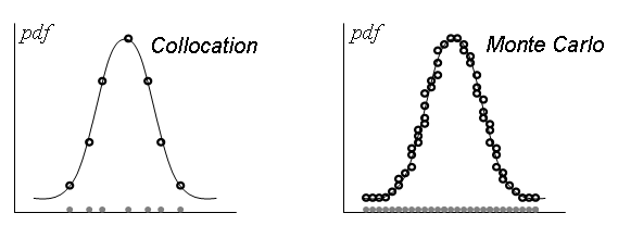
Table 20.3: Roots of Hermite Polynomials
|
j |
Hj(x) |
Location of zeros (in the order of their probability) |
|---|---|---|
|
1 |
x |
0 |
|
2 |
x2 - 1 |
±1 |
|
3 |
x3 - 3x |
0, ±1.7321 |
|
4 |
x4 - 6x2 + 3 |
±0.7420, ±2.3344 |
|
5 |
x5 - 10x3 + 15x |
0, ±1.3556, ±2.8570 |
|
6 |
x6 - 15x4 + 45x2 - 15 |
±0.6167, ±1.8892, ±3.3243 |
|
7 |
x7 - 21x5 + 105x3 - 105x |
0, ±1.1544, ±2.3668, ±3.7504 |
|
8 |
x8 - 28x6 + 210x4 - 420x2 + 105 |
±0.5391, ±1.6365, ±2.8025, ±4.1445 |
|
9 |
x9 - 36x7 + 378x5 - 1260x3 + 945x |
0, ±1.0233, ±2.0768, ±3.2054, ±4.5127 |
[3] Parts of Figure 20.1: Comparison of collocation points for normal PDF and sampling points for Monte Carlo method: (a) Location of the collocation points that correspond to roots of the Hermite polynomial expansion for a normal probability distribution function (PDF) and (b) sampling points necessary using a Monte Carlo method to achieve the same resolution of the PDF