Two current mixing models are considered: the modified Curl's mixing model [81] and the linear-mean-square-estimation (LMSE) model. Briefly, we summarize the expressions of these mixing models here. Detailed descriptions of these models can be found in the corresponding references.
 | (10–6) |
where  is the transitional probability defined as
  for
for  otherwise
  .
.
The Interaction-by-Exchange-with-the-Mean ( IEM) or the Linear-Mean-Square-Estimation ( LMSE) model [82] is shown in Equation 10–7
 | (10–7) |
where  is a constant parameter for the model.
Chen[79] derived analytical forms of unmixedness as a function of mixing time scale for the two mixing models. These analytical functions serve as a base for validating the PaSR code. The unmixedness or the segregation variable is a parameter used to quantify the unmixed nature, and its definition is given as
 | (10–8) |
Where  is the mixture fraction and
  and
and  denote density-weighted average and fluctuation, respectively. The
definition guarantees that the unmixedness is bounded by zero and one, which corresponds to
completely segregated and perfectly mixed states, respectively. The theoretical values of the
unmixedness at the statistically stationary state for the two mixing models are:
denote density-weighted average and fluctuation, respectively. The
definition guarantees that the unmixedness is bounded by zero and one, which corresponds to
completely segregated and perfectly mixed states, respectively. The theoretical values of the
unmixedness at the statistically stationary state for the two mixing models are:
 | (10–9) |
 | (10–10) |
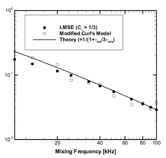
When  , the two mixing models should produce identical levels of unmixedness for a
given mixing time scale. Figure 10.1: Unmixedness vs. mixing frequency for PaSR of stoichiometric H2
/air mixture with 1 ms residence time
shows the unmixedness versus mixing
frequency from simulations of a pure mixing problem for
, the two mixing models should produce identical levels of unmixedness for a
given mixing time scale. Figure 10.1: Unmixedness vs. mixing frequency for PaSR of stoichiometric H2
/air mixture with 1 ms residence time
shows the unmixedness versus mixing
frequency from simulations of a pure mixing problem for  . The numerical results of Ansys Chemkin show excellent agreement with the
theoretical values.
. The numerical results of Ansys Chemkin show excellent agreement with the
theoretical values.
Figure 10.1: Unmixedness vs. mixing frequency for PaSR of stoichiometric H2 /air mixture with 1 ms residence time