The conservation equations defining the boundary-value system that we solve are stated below.

(15–1)

(15–2)

(15–3)

(15–4)

Figure 15.1: Sketch of the infinite-radius disk and inlet boundary conditions

(15–5)

(15–6)

(15–7)

The above equations can be solved as either a steady-state problem or time-accurate transient. For a steady-state solution, the solution is sought to the above equations where the transient terms on the left-hand side of the equations are zero. The steady-state algorithm is discussed further in the Numerical Solution Methods .

In the governing equations the independent variables are , the distance normal to the disk surface, and , time. The dependent variables are the velocities, the temperature , the gas-phase species mass fractions , and the surface-species site fractions . The axial velocity is , and the radial and circumferential velocities are scaled by the radius as and , respectively. The mass density is given by and the specific heats by . The molecular weight and specific enthalpy for species are given by and . The viscosity and thermal conductivity are given by and . The universal gas constant is . The chemical production rate of species by the gas-phase reaction is resumed to result from a system of elementary chemical reactions that proceed according to the law of mass action. The chemical production rate of species by surface reaction is given by . is the number of gas-phase species and is the number of surface species, not including bulk-phase species. The factor is the surface site density for site type . The details of the chemical reaction rate formulation can be found in Gas-phase Chemical Rate Expressions and Surface Chemical Rate Expressions . Details of the transport property (that is, viscosities, thermal conductivities and diffusion coefficients) formulation can be found in Gas-phase Species Transport Properties .

The term in the radial momentum equation is taken to be constant and its value is computed as an eigenvalue of the problem. The pressure is assumed to be composed of two parts: an average thermodynamic pressure that is taken to be constant, and a spatially varying component that appears in the radial momentum equation, see Equation 15–2 (c.f. Paolucci [120]).

The "surface-species conservation" equation states simply that in steady state the surface composition does not change. In some sense it could be considered a (possibly complex) boundary condition on the gas-phase system. However, because the surface composition is determined as part of the solution, Equation 15–7 should be considered part of the system of governing equations.

Provisions are made for dealing with the transport properties at the mixture-averaged (Fickian) level or at the full multicomponent level. At the mixture-averaged level, each species diffusion velocity is calculated in terms of a diffusion coefficient and a species gradient,

(15–8)

where,

(15–9)

At the multicomponent level, the diffusion velocities are given as

(15–10)

Both formulations have an ordinary diffusion component and may have a thermal diffusion component ( Soret effect). In these expressions, is the mole fraction for the k th species, is the binary diffusion coefficient matrix, is the matrix of ordinary multicomponent diffusion coefficients, and is the thermal diffusion coefficient for the k th species. Thermal diffusion often plays an important role in CVD problems. In the presence of strong temperature gradients, thermal diffusion causes high molecular-weight species in a low molecular-weight carrier to diffuse rapidly toward the low-temperature region.[35] The multicomponent and mixture transport properties are evaluated from the pure species properties using the averaging procedures as discussed in Gas-phase Species Transport Properties .

Mass conservation requires that . However, a consequence of using the Fickian mixture-averaged diffusion coefficient defined in Equation 15–9 to define a diffusion velocity in Equation 15–8 is that mass is not always conserved, that is, . Therefore, at this level of closure of the transport formulation, some corrective measures must be taken. The user has several options. One is for the program to apply an ad hoc Correction Velocity, defined as

(15–11)

When this correction velocity (independent of species ) is added to all the species diffusion velocities as computed from Equation 15–8 , mass conservation is assured.

Another option is to account for the deficiencies of the mixture-averaged closure of the multicomponent transport problem and to assure mass conservation is to solve only gas-phase species conservation equations and determine the remaining mass fraction by requiring (Trace option). The mixture-averaged transport closure is asymptotically correct in the trace-species limit. In cases where one species is present in large excess (such as a carrier gas in a CVD reactor), this is a reasonable option.

The carrier gas composition is conventionally determined as

(15–12)

The default for this option is to consider the last-named gas-phase species in the Gas-phase Kinetics input () as the species for which a conservation equation is not solved. Since the last species may not always be the most abundant species, a further option provides for dynamically determining the largest species concentration at each mesh point and removing its conservation equation from the system of equations (Reorder option in the User Interface).

The source term in the thermal energy equation is a spatially distributed thermal energy source that we assume is in the form of a Gaussian:

(15–13)

To use this expression, the user is expected to specify three parameters: , and . The parameter is the total energy integrated over its full spatial extent. Implicit in Equation 15–13 is the fact that

(15–14)

The distribution is centered at and is the half-width of the distribution. (The integral of from to includes 95% of the total added energy .)

The disk boundary condition becomes relatively complex in the presence of heterogeneous surface reactions. The gas-phase mass flux of each species to the surface is balanced by the creation or depletion of that species by surface reactions, that is,

(15–15)

The gas-phase mass flux of species at the surface is a combination of diffusive and convective processes,

(15–16)

where is the bulk normal fluid velocity at the surface and is the diffusion velocity of the k th species. The bulk normal fluid velocity at the surface is computed from the surface reaction rates summed over all the gas-phase species ,

(15–17)

Even though the susceptor surface is solid, there is a bulk fluid velocity into the surface (the Stefan velocity) that accounts for the mass of solids deposited. This bulk velocity at the surface is usually small, and thus the boundary movement due to the deposition is neglected. That is, the problem is solved in a fixed spatial domain. While the surface growth rate is predicted, the computational domain is not adjusted to account for small changes resulting from surface growth.

There are two options for treating the thermal-energy boundary condition on the deposition surface. The first is to simply specify the surface temperature. If the temperature is controlled or measured directly, this option is usually the one of choice. However, some problems require that the surface temperature be predicted as part of the solution. The appropriate boundary condition is derived from a surface energy balance. Exothermicity (or endothermicity) of surface reactions contributes to the energy balance at an interface. Diffusive and convective fluxes in the gas-phase are balanced by thermal radiative and chemical heat release at the surface. This balance is stated as

(15–18)

In the radiation term, is the Stefan-Boltzmann constant, is the surface emissivity, and is the temperature to which the surface radiates. The summation on the right-hand side runs over all surface and bulk species. and are the Surface Kinetics notations for the indices that identify the first surface species and the last bulk species. By substituting Equation 15–15 and Equation 15–16 into Equation 15–18 , the energy balance can be written in a more compact form as

(15–19)

The reaction-rate summation on the right-hand side runs over all species, including the gas-phase species. The term presents an energy source in the surface itself, such as might be generated by resistance heating.

The Surface Kinetics Pre-processor requires as input the mass densities of the bulk species. These densities are used to convert the rate of production of a bulk species (in moles/cm² /sec) into a thickness growth rate (in cm/sec). The needed relationship is

(15–20)

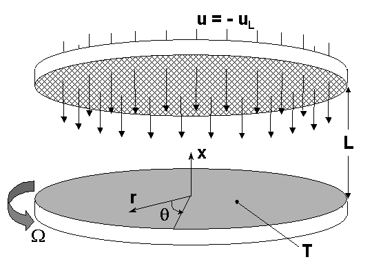
When solving for the flow induced by the rotation of a disk in an infinite, otherwise quiescent fluid, the axial velocity at is part of the solution. However, for the case corresponding to injection of the gas through a non-rotating porous surface, u is the specified inlet velocity at height . This gives us the flexibility of either "forcing" or "starving" the inlet flow compared to the natural flow induced by the spinning disk itself. It is always necessary to specify the inlet velocity in the case of a stagnation-point flow.

The other boundary conditions on the fluid flow fields are relatively simple. The temperature at (the reactor inlet) is specified. Normally, the radial and circumferential velocities are zero at . A linearly varying radial velocity or a specified spin rate may also be specified at . In these cases, or , where and are specified parameters. The radial velocity on the disk is zero, and the circumferential velocity is determined from the spinning rate . For the species composition at the inlet boundary, the default formulation is to solve the following flux balance:

(15–21)

where is the species mass fraction specified for the inflow. The user may also opt to fix the species composition (that is, ), by specifying the option in the User Interface to fix the inlet composition rather than the inlet flux.