


This tutorial includes:
- 23.1. Tutorial Features
- 23.2. Overview of the Problem to Solve
- 23.3. Preparing the Working Directory
- 23.4. Setting Up the Project
- 23.5. Defining the Geometry Using Ansys BladeGen
- 23.6. Defining the Mesh
- 23.7. Defining the Case Using CFX-Pre
- 23.8. Obtaining the Solution Using CFX-Solver Manager
- 23.9. Viewing the Results Using CFD-Post
- 23.10. Simulating the Structural Performance Using Static Structural
Note: Because this tutorial makes use of Ansys BladeGen, it must be run on a Windows-based machine.
This tutorial addresses the following features:
Component | Feature | Details |
|---|---|---|
Ansys BladeGen | Geometry | Transfer of geometry to Ansys TurboGrid and Mechanical Model |
Ansys TurboGrid | Mesh | Shroud Tip defined by Profile |
ATM Optimized | ||
Mechanical Model | Mesh | Virtual Topology |
Edge Sizing | ||
Face Meshing | ||
Sweep Method | ||
CFX-Pre | User Mode | Turbo mode |
General mode | ||
Machine Type | Centrifugal Compressor | |
Component Type | Rotating | |
Analysis Type | Steady State | |
Domain Type | Fluid Domain | |
Solid Domain | ||
Fluid Type | Air Ideal Gas | |
Boundary Template | P-Total Inlet Mass Flow Outlet | |
Flow Direction | Cylindrical Components | |
Solid Type | Steel | |
Heat Transfer | Thermal Energy | |
Domain Interface | Fluid Fluid | |
Fluid Solid | ||
Timestep | Physical Timescale | |
CFD-Post | Report | Computed Results Table |
Blade Loading Span 50 | ||
Streamwise Plot of Pt and P | ||
Velocity Streamlines Stream Blade TE | ||
Static Structural | Static Structural Analysis | Importing CFX pressure data |
Importing CFX temperature data | ||
Fixed Support | ||
Rotationally-induced inertial effect | ||
Static Structural Solutions | Equivalent Stress (von-Mises) | |
Total Deformation |
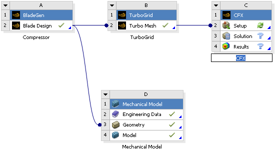
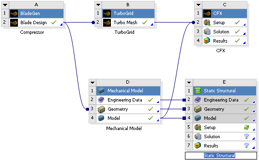
This tutorial makes use of several Ansys software components to simulate the aerodynamic and structural performance of a centrifugal compressor.
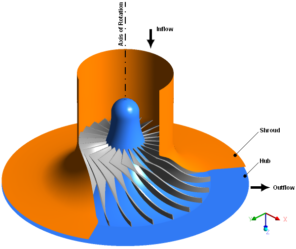
The compressor has 24 blades that revolve about the Z axis at 22360 RPM. A clearance gap exists between the blades and the shroud of the compressor. The outer diameter of the blade row is approximately 40 cm.
To begin analysis of the aerodynamic performance, a mesh will be created in both Ansys TurboGrid and the Mechanical application using an existing design that is to be reviewed beforehand in Ansys BladeGen. Once the meshes have been created, initial parameters defining the aerodynamic simulation will be set in CFX-Pre and then solved in CFX-Solver. The aerodynamic solution from the solver will then be processed and displayed in CFD-Post.
You will then use the Mechanical application to simulate structural stresses and deformation on the blade due to pressure and temperature loads from the aerodynamic analysis and rotationally-induced inertial effects. You will view an animation that shows the resulting blade distortion.
If this is the first tutorial you are working with, it is important to review the following topics before beginning:
Create a working directory.
Ansys CFX uses a working directory as the default location for loading and saving files for a particular session or project.
Download the
centrifugal_compressor.zipfile here .Unzip
centrifugal_compressor.zipto your working directory.Ensure that the following tutorial input file is in your working directory:
Centrifugal_Compressor.bgd
Start Ansys Workbench by clicking the Start menu then selecting All Programs > Ansys 2024 R2 > Workbench 2024 R2.
From the main menu, select File > Save As.
In the Save As dialog box, browse to the working directory and set File name to
Compressor.Click .
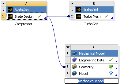
In the Toolbox view, expand Component Systems and double-click BladeGen.
In the Project Schematic view, a BladeGen system opens and is ready to be given a name.
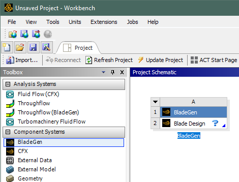
In the name field, type
Compressorand then either press Enter or click outside the name field to end the rename operation.If you need to begin a new rename operation, right-click the BladeGen cell (A1) and select Rename.
Now that renaming systems has been demonstrated, most of the other systems involved in this tutorial will simply use default names.
Change the Blade Design cell properties as follows:
In the Project Schematic view, in the BladeGen system, right-click the Blade Design cell and select Properties.
The properties view shows properties that control how the geometry is exported to downstream systems.
In the properties view, clear the Merge Blade Topology and Create Fluid Zone check boxes.
By clearing the Create Fluid Zone check box, you are specifying that only the blade geometry, and not the volume around the blade, should be sent to downstream cells.
Set Shroud Clearance to
Relative Layer.This will make sure the tip clearance layer is not part of the geometry when it is transferred to the Mechanical application.
The properties should appear as follows:
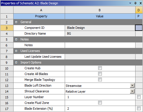
You now have a BladeGen system that contains a Blade Design cell; the latter is presently in an unfulfilled state, as indicated by the question mark. In the next section, you will fulfill the cell requirements by loading the provided geometry file. In general, you could also fulfill the cell requirements by creating a new geometry.
In this section, you will load the geometry from the provided .bgd file, and then review the blade design using Ansys BladeGen. BladeGen is a geometry-creation tool specifically designed for turbomachinery blades.
In the Project Schematic view, in the BladeGen system, right-click the Blade Design cell and select Edit or double-click the cell.
BladeGen opens.
In BladeGen, in the main menu, select File > Open.
In the Open dialog box, browse to the working directory and select the file Centrifugal_Compressor.bgd.
Click Open.
Observe the blade design shown in BladeGen.
Quit BladeGen.
To do this, in the main menu, select File > Exit.
In the Project Schematic view, the Blade Design cell now displays a green check mark to indicate that the cell is up-to-date. This means that you now have a geometry for the centrifugal compressor that is ready to be used for meshing purposes.
In the next section, you will create a CFD-compatible mesh based on this geometry.
You will create a mesh in both Ansys TurboGrid and the Mechanical application. TurboGrid will create a CFD mesh that will be part of the fluid domain. The Mechanical application will generate the solid blade mesh that is required for solving for the volumetric temperature in the blade.
TurboGrid is a mesh creation tool specifically designed for turbomachinery blades. In this section, you will use TurboGrid to produce a CFD-compatible mesh based on the centrifugal compressor geometry.
In the BladeGen system, right-click the Blade Design cell and select Transfer Data To New > TurboGrid.
A TurboGrid system opens and is ready to be given a name.
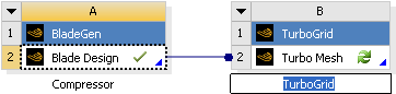
Press Enter to accept the default name.
The Turbo Mesh cell displays a pair of green curved arrows to indicate that the cell has not received the latest upstream data. Normally, you would right-click such a cell and select Refresh to transfer data from the upstream cell. However, for a newly-added Turbo Mesh cell and whenever TurboGrid is not open, this action is not necessary because TurboGrid always reads the upstream cell data upon starting up.
If you were to refresh the Turbo Mesh cell, it would show a question mark to indicate that, although the cell's inputs are current, further attention is required in order to bring the cell to an up-to-date status; that further action would typically be to run TurboGrid and produce a mesh with it.
In the TurboGrid system, right-click the Turbo Mesh cell and select Edit.
TurboGrid opens.
The next several sections guide you through the steps to create the CFD mesh.
For this compressor, the shroud is stationary and requires a clearance gap between the blade and shroud. Define the tip of the blade using the second blade profile in the blade geometry.
In TurboGrid, in the object selector, right-click
Geometry>Blade Set>Shroud Tipand select Edit.In the object editor, configure the following setting(s):
Tab
Setting
Value
Shroud Tip
Override Upstream Geometry Options
(Selected)
Tip Option
Profile Number
Tip Profile
2
Click Apply.
This defines the shroud tip of the blade (the surface of the blade that is nearest to the shroud).
Now that the geometry is defined, create the topology and mesh:
Right-click
Topology Setand turn off Suspend Object Updates.The topology and 3D mesh are generated.
The Mesh Data settings control the number
and distribution of mesh elements.
In the object selector, right-click
Mesh Dataand select Edit.Alternatively, in the toolbar, click Edit Mesh Data
 .
.In the object editor, configure the following setting(s):
Tab
Setting
Value
Mesh Size
Method
Target Passage Mesh Size
Node Count
Medium (100000)
Inlet Domain
(Selected)
Outlet Domain
(Selected)
Passage
Spanwise Blade Distribution Parameters
> Method
Element Count and Size
Spanwise Blade Distribution Parameters
> # of Elements
25
Spanwise Blade Distribution Parameters
> Const Elements
11
Inlet
Inlet Domain
> Define By
Target Number of Elements
Inlet Domain
> # of Elements
50
Outlet
Outlet Domain
> Define By
Target Number of Elements
Outlet Domain
> # of Elements
25
Click .
Select File > Close TurboGrid.
Return to the Project Schematic view.
A mesh is required for the solid blade geometry for CFX-Solver to solve for the volumetric temperature. This volumetric temperature will later be exported to Static Structural to calculate the stresses on the blade. In this section, you will use the Mechanical application to produce a solid blade mesh.
In the BladeGen system, right-click the Blade Design cell and select Transfer Data To New > Mechanical Model.
A Mechanical Model system opens and is ready to be given a name.
Press Enter to accept the default name.
In the Mechanical Model system, right-click the Geometry cell and select Update.
Ansys DesignModeler runs in the background, and imports the geometry from the BladeGen system.
Right-click the Model cell and select Edit.
The Mechanical application opens.
The next several sections guide you through the steps to create the mesh.
In the Mechanical application, in the Outline tree view, select
Project>Model (C4)>Mesh.In the details view, configure the following setting(s):
Group
Control
Value
Defaults
Physics Preference
Mechanical
The geometry has unnecessary small faces and edges, as shown in Figure 23.1: Small Face at the Leading Edge of the Blade, which can influence the mapping of the mesh. Creating a virtual topology of virtual faces and edges will fix the problem by letting the Mechanical application ignore these geometry flaws.
In the Outline tree view, right-click
Project>Model (C4)and select Insert > Virtual Topology.Right-click
Project>Model (C4)>Virtual Topologyand select Generate Virtual Cells.This will automatically create most of the virtual cells for you. You will have to make the rest of the virtual cells manually.
In the viewer, right-click and select View > Back.
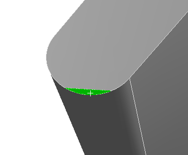
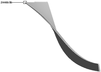
Select the long thin face of the blade that is shown highlighted in green in Figure 23.2: Back View of the Blade.
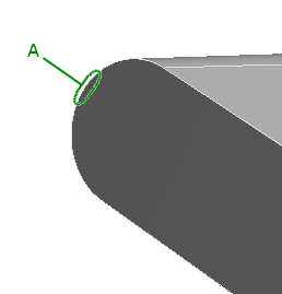
Zoom in on the trailing edge as shown in Figure 23.2: Back View of the Blade.
Hold Ctrl and select the small face at the trailing edge beside the long thin face shown in Figure 23.3: Small Face at the Trailing Edge of the Blade.
In the viewer, right-click and select Insert > Virtual Cell.
In the viewer, right-click and select View > Bottom.
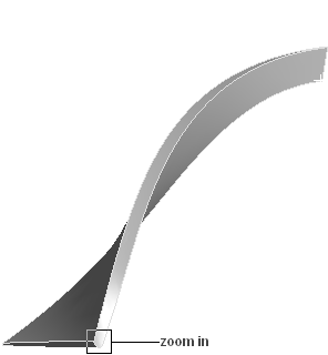
Zoom in on the leading edge as shown in Figure 23.4: Bottom View of the Blade.
Hold Ctrl and select the three edges marked "A", "B" and "C" in Figure 23.5: Three Edges at the Leading Edge of the Blade.
In the viewer, right-click and select Insert > Virtual Cell.


You will now apply local mesh sizing on four edges at the blade tip.
In the Outline tree view, right-click
Project>Model (C4)>Meshand select Insert > Sizing.In the viewer, right-click and select View > Back so that the model is oriented similar to the one shown in Figure 23.2: Back View of the Blade.
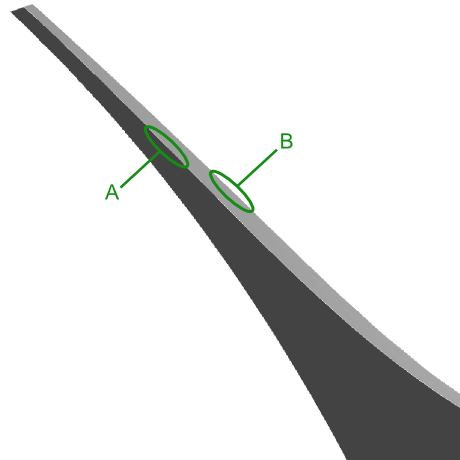
Hold Ctrl and select the two edges marked "A" and "B" in Figure 23.6: Two Edges on the Back of the Blade.
In the details view, click in the field beside Scope > Geometry.
The field beside Scope > Geometry should now display
2 Edges. You have now chosen the two edges on which to apply the Sizing control.Configure the following setting(s):
In the Outline tree view, right-click
Project>Model (C4)>Meshand select Insert > Sizing.Zoom in on the trailing edge as indicated in Figure 23.2: Back View of the Blade.
Select the edge marked "C" in Figure 23.7: Edge on the Trailing Edge of the Blade.
In the details view, click in the field beside Scope > Geometry.
The field beside Scope > Geometry should now display
1 Edge.Configure the following setting(s):
Setting
Value
Definition
> Type
Number of Divisions
Definition
> Number of Divisions
3
Definition
> Behavior
Hard
Definition
> Bias Type
No Bias
In the Outline tree view, right-click
Project>Model (C4)>Meshand select Insert > Sizing.In the viewer, right-click and select View > Top.
Zoom in on the leading edge as shown in Figure 23.8: Top View of the Blade.
Select the edge marked "A" in Figure 23.9: Leading Edge of the Blade.
In the details view, click in the field beside Scope > Geometry.
The field beside Scope > Geometry should now display
1 Edge.Configure the following setting(s):
Setting
Value
Definition
> Type
Number of Divisions
Definition
> Number of Divisions
3
Definition
> Behavior
Hard
Definition
> Bias Type
____ __ _ __ ____
Definition
> Bias Factor
3

You will now introduce a Face Meshing control on the blade tip that will generate a structured mesh based on the Sizing controls that you just defined.
In the Outline tree view, right-click
Project>Model (C4)>Meshand select Insert > Face Meshing.Select the virtual face at the top of the blade where you just defined the Sizing controls (the face that is at the forefront of the displayed geometry in Figure 23.9: Leading Edge of the Blade).
In the details view, click in the field beside Scope > Geometry.
The field beside Scope > Geometry should now display
1 Face. This is the face at the blade tip.
In the Outline tree view, right-click
Project>Model (C4)>Meshand select Show > Sweepable Bodies.This will select the sweepable bodies in the viewer; in this case, it is the whole blade geometry.
Right-click
Project>Model (C4)>Meshand select Insert > Method.In the details view, set Definition > Method to
Sweep.Set Definition > Src/Trg Selection to
Manual Source and Target.In the details view, click the field beside Definition > Source where it says
No Selection.Two buttons appear in the field: Apply and Cancel.
Select the virtual face at the top of the blade where you just defined the Face Meshing control (the face that is at the forefront of the displayed geometry in Figure 23.9: Leading Edge of the Blade).
In the details view, click in the field beside Definition > Source.
The face has been selected as the source for the sweep method.
Follow a similar procedure for Definition > Target to set the bottom virtual face of the blade as the target for the sweep method (the face that is attached to the hub and opposite to the virtual face at the top of the blade).
Configure the following setting(s):
Setting
Value
Definition
> Type
Number of Divisions
Definition
> Sweep Num Divs
15
Definition
> Sweep Bias Type
_ __ ____ __ _
Definition
> Sweep Bias [a]
10
In the Outline tree view, right-click
Project>Model (C4)>Meshand select Update.After a few moments, the mesh is generated. You will now observe the mesh statistics.
Click
Project>Model (C4)>Mesh.In the details view, expand Statistics.
Note the node and element count.
Note: To obtain better results, the mesh would require a greater number of elements, especially through the thickness of the blade; however, the current mesh is sufficient for the purposes of this tutorial.
Set Mesh Metric to any option and observe the mesh metric bar graph that appears.
Quit the Mechanical application.
To do this, select the File tab and select Close Mechanical.
Return to the Project Schematic view.
This section involves using CFX-Pre in Ansys Workbench. CFX-Pre is a CFD physics preprocessor that has a Turbo mode facility for setting up turbomachinery CFD simulations. In this section, you will use CFX-Pre in Turbo mode to define a CFD simulation based on the centrifugal compressor mesh that you created earlier. Later in General mode, you will create a solid domain for the blade and make a fluid-solid interface.
In the TurboGrid system, right-click the Turbo Mesh cell and select Transfer Data To New > CFX.
A CFX system opens and is ready to be given a name.
Press Enter to accept the default name.
Drag the Model cell of the Mechanical Model system to the Setup cell of the CFX system.
In the Mechanical Model system, right-click the Model cell and select Update.
The Mesh cell now displays a green check mark to indicate that the cell is up to date. This means that the blade mesh is available for use in the CFD simulation. The Setup cell displays a pair of green curved arrows to indicate that the cell has not received the latest upstream data. Since you have not yet opened CFX-Pre, you can disregard the cell status; CFX-Pre will automatically read the upstream cell data upon starting up from this cell for the first time.
In the CFX system, right-click the Setup cell and select Edit.
CFX-Pre opens.
The next several sections guide you through the steps to create the CFD simulation.
You will define the fluid domain, boundaries and interfaces in Turbo mode.
In CFX-Pre, in the main menu, select Tools > Turbo Mode.
In the Basic Settings panel, configure the following setting(s):
Setting
Value
Machine Type
Centrifugal Compressor
Axes
> Rotation Axis
Z
Analysis Type
> Type
Steady State
Leave the other settings at their default values.
Click Next.
In the Component Definition panel, right-click
Componentsand select Add Component.In the New Component dialog box, set Name to
R1and Type toRotating.Note: If the Automatic Default Domain option in CFX-Pre is selected, a domain with the name
R1will already be present under the Component Definition panel. In this case, you do not need to create a new domain, and you can continue by editing the existingR1componentClick .
Select
Components>R1and configure the following setting(s):Setting
Value
Component Type
> Type
Rotating
Component Type
> Value
22360 [rev min^-1]
Mesh
> Available Volumes
> Volumes
Inlet, Outlet, Passage Main
Wall Configuration
(Selected)
Wall Configuration
> Tip Clearance at Shroud
> Yes
(Selected)
Leave the other settings at their default values.
Note: When a component is defined, Turbo mode will automatically select a list of regions that correspond to certain boundary types. This information should be reviewed under Region Information to ensure that all is correct.
Click Next.
You will now set the properties of the fluid domain and some solver parameters.
In the Physics Definition panel, configure the following setting(s):
Setting
Value
Fluid
Air Ideal Gas
Model Data
> Reference Pressure
1 [atm]
Model Data
> Heat Transfer
Total Energy
Model Data
> Turbulence
k-Epsilon
Inflow/Outflow Boundary Templates
> P-Total Inlet Mass Flow Outlet
(Selected)
Inflow/Outflow Boundary Templates
> Inflow
> P-Total
0 [atm]
Inflow/Outflow Boundary Templates
> Inflow
> T-Total
20 [C]
Inflow/Outflow Boundary Templates
> Inflow
> Flow Direction
Cylindrical Components
Inflow/Outflow Boundary Templates
> Inflow
> Inflow Direction (a,r,t)
1, 0, 0
Inflow/Outflow Boundary Templates
> Outflow
> Mass Flow
Per Component
Inflow/Outflow Boundary Templates
> Outflow
> Mass Flow Rate
0.167 [kg s^-1]
Solver Parameters
(Selected)
Solver Parameters
> Convergence Control
Physical Timescale
Solver Parameters
> Physical Timescale
0.0002 [s]
Leave the other settings at their default values.
Click .
CFX-Pre will try to create appropriate interfaces using the region names presented previously under Region Information in the Component Definition panel.
In the Interface Definition panel, verify that each interface is set correctly; select an interface listed in the tree view and then examine the associated settings (shown in the lower portion of the panel) and highlighted regions in the viewer.
If no regions appear highlighted in the viewer, ensure that highlighting is turned on in the viewer toolbar.
Click .
CFX-Pre will try to create appropriate boundary conditions using the region names presented previously under Region Information in the Component Definition panel.
In the Boundary Definition panel, verify that each boundary is set correctly; select a boundary listed in the tree view and then examine the associated settings and highlighted regions.
Note: Later, you will delete
R1 Bladeboundary in General mode after creating a fluid-solid interface at the blade.Click .
You will need to create a solid domain for the blade followed by making a fluid-solid interface in General mode.
In the Outline tree view, right-click
Simulation>Flow Analysis 1and select Insert > Domain.In the Insert Domain dialog box, set Name to
Solid Blade.Click .
Configure the following setting(s) of
Solid Blade:Tab
Setting
Value
Basic Settings
Location and Type
> Location
B24 [a]
Location and Type
> Domain Type
Solid Domain
Solid Definitions
Solid 1
Solid Definitions
> Solid 1
> Material
Steel
Domain Models
> Domain Motion
> Option
Rotating
Domain Models
> Domain Motion
> Angular Velocity
22360 [rev min^-1]
Domain Models
> Domain Motion
> Axis Definition
> Option
Coordinate Axis
Domain Models
> Domain Motion
> Axis Definition
> Rotation Axis
Global Z
Solid Models
Heat Transfer
> Option
Thermal Energy
Click .
You do not need to create any boundaries for the solid domain because the interfaces will make the boundaries for you. The only surface that must be specified is the bottom of the blade at the hub. You will review the default boundary because it will later represent the bottom of the blade after all the interfaces have been specified.
In the Outline tree view, right-click
Simulation>Flow Analysis 1>Solid Blade>Solid Blade Defaultand select Edit.Configure the following setting(s) of
Solid Blade Default:Tab
Setting
Value
Basic Settings
Boundary Type
Wall
Boundary Details
Heat Transfer
> Option
Adiabatic
Click .
An interface is required between the two meshes at the blade surface.
In the Outline tree view, right-click
Simulation>Flow Analysis 1and select Insert > Domain Interface.In the Insert Domain Interface dialog box, set Name to
R1 to Solid Blade.Click .
Configure the following setting(s) of
R1 to Solid Blade:Tab
Setting
Value
Basic Settings
Interface Type
Fluid Solid
Interface Side 1
> Domain (Filter)
R1
Interface Side 1
> Region List
BLADE
Interface Side 2
> Domain (Filter)
Solid Blade
Interface Side 2
> Region List
F26.24,F28.24,F30.24, F31.24,F49.24 [a]
Interface Models
> Option
General Connection [b]
Mesh Connection
Mesh Connection Method
> Mesh Connection
> Option
Automatic
Click .
A warning message appears notifying that the region for
R1 Bladehas already been specified as a boundary.In the Outline tree view, right-click
Simulation>Flow Analysis 1>R1>R1 Bladeand select Delete.The warning message disappears.
Quit CFX-Pre.
To do this, in the main menu, select File > Close CFX-Pre.
Return to the Project Schematic view.
Generate a solution for the CFD simulation that you just prepared:
In the CFX system, right-click the Solution cell and select Update.
After some time, a CFD solution will be generated. If the progress indicator is not visible, you can display it by clicking
 or, to see detailed output, right-click the Solution cell and select Display Monitors.
After the solution has been generated, return to the Project Schematic view.
CFD-Post enables you to view the results in various ways, including tables, charts, and figures. You can present the results in the form of a report that can be viewed in CFD-Post, or exported for viewing in another application.
Create a report and examine some of the results as follows:
In the CFX system, right-click the Results cell and select Edit.
CFD-Post opens.
In CFD-Post, select File > Report > Report Templates.
In the Report Templates dialog box, select Centrifugal Compressor Rotor Report and click .
In the Outline tree view, right-click
Report>Compressor Performance Results Tableand select Edit.This table presents measures of aerodynamic performance including required power and efficiencies.
Right-click
Report>Blade Loading Span 50and select Edit.This is a plot of the pressure vs. streamwise distance along both the pressure and suction sides of the blade at mid-span.
Right-click
Report>Streamwise Plot of Pt and Pand select Edit.This is a plot of the streamwise variation of pressure and total pressure.
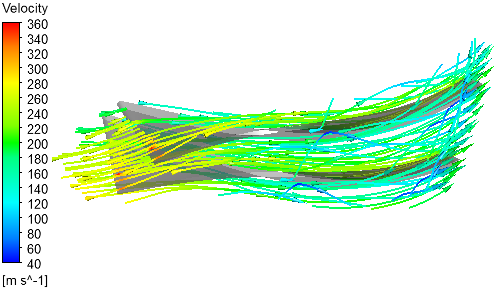
Right-click
Report>Velocity Streamlines Stream Blade TE Viewand select Edit.This is a trailing-edge view of the streamlines that start upstream of the blade.
To view a full report, click the Report Viewer tab found near the bottom right of the window.
A report will be generated that includes all figures available under
Reportin the tree view. This report can be viewed in CFD-Post or published to be viewed externally as an .html or .txt file.Note that if you have visited the Report Viewer before loading the template, or have otherwise made any changes to the report definition after first viewing the report, you need to click
 in the Report Viewer to update the report as
displayed.
in the Report Viewer to update the report as
displayed.Quit CFD-Post.
To do this, in the main menu, select File > Close CFD-Post.
Return to the Project Schematic view.
This section describes the steps required to simulate structural stresses and deformation on the blade due to pressure and temperature loads from the aerodynamic analysis.
Expand Analysis Systems in the Toolbox view and drag Static Structural to the Model cell of the Mechanical Model system in the Project Schematic view.
In the Project Schematic view, a Static Structural system opens and is ready to be given a name.
Press Enter to accept the default name.
Drag the Solution cell of the CFX system to the Setup cell of the Static Structural system.
This makes the CFD solution data available for use in the structural analysis.
In the Static Structural system, right-click the Setup cell and select Edit.
The Mechanical application opens.
The next several sections guide you through the steps to create a structural simulation with and without rotationally-induced inertial effects.
This Static Structural system will be used to create the simulation without the inertial loads.
In the Mechanical application, in the Outline tree view, right-click
Project>Model (D4, E4)>Static Structural (D5)>Imported Load (C3)and select Insert > Pressure.After a short time,
Project>Model (D4, E4)>Static Structural (D5)>Imported Load (C3)>Imported Pressurewill appear and will be selected.In the details view, click the field beside Scope > Geometry where it says
No Selection.In the viewer, right-click and select Select All.
Alternatively, in the main menu, select Edit > Select All.
In the viewer, right-click and select View > Bottom.
Hold Ctrl and select the long thin face of the blade that is at the forefront of the displayed geometry.
This is the surface that is attached to the hub.
In the details view, click in the field beside Scope > Geometry.
The field beside Scope > Geometry should now display
5 Faces. You have now chosen the solid model surface onto which the CFD pressure data will be applied.Set Transfer Definition > CFD Surface to
R1 to Solid Blade Side 1.You have now chosen the CFD boundary from which to get the CFD pressure data. You will do the same for the body temperature.
In the Outline tree view, right-click
Project>Model (D4, E4)>Static Structural (D5)>Imported Load (C3)and select Insert > Body Temperature.In the details view, click the field beside Scope > Geometry where it says
No Selection.In the viewer, right-click and select Select All.
In the details view, click in the field beside Scope > Geometry.
The field beside Scope > Geometry should now display
1 Body. You have now chosen the solid model onto which the CFD temperature data will be applied.Set Transfer Definition > CFD Domain to
Solid Blade.You have now chosen the CFD domain from which to get the CFD temperature data.
In the Outline tree view, right-click
Project>Model (D4, E4)>Static Structural (D5)>Imported Load (C3)and select Import Load.Wait for the Mechanical application to map the loads.
To verify that the pressure and temperature data were applied correctly to the blade, inspect
Imported Pressure>Imported Load Transfer SummaryandImported Body Temperature>Imported Load Transfer SummaryunderProject>Model (D4, E4)>Static Structural (D5)>Imported Load (C3).The slight discrepancy shown in the load transfer summary for the imported pressure is due to a difference in the TurboGrid and Mechanical mesh. In general, accurate load mapping requires that the surface mesh elements match.
In the Outline tree view, right-click
Project>Model (D4, E4)>Static Structural (D5)and select Insert > Fixed Support.In the viewer, right-click and select View > Bottom.
Select the long thin face of the blade that is at the forefront of the displayed geometry.
In the details view, click in the field beside Scope > Geometry.
The face that you selected is now connected to the hub.
In the Outline tree view, right-click
Project>Model (D4, E4)>Static Structural (D5)>Solution (D6)and select Insert > Stress > Equivalent (von-Mises).Right-click
Project>Model (D4, E4)>Static Structural (D5)>Solution (D6)and select Insert > Deformation > Total.Right-click
Project>Model (D4, E4)>Static Structural (D5)>Solution (D6)and select Solve.Alternatively, in the toolbar, click
 .
.Wait for the solver to finish.
Select
Project>Model (D4, E4)>Static Structural (D5)>Solution (D6)>Equivalent Stressto prepare to examine the von-Mises stress results.In the Graph view, click Play
 to animate the physical deformation
of the blade along with the associated von-Mises stress results.
to animate the physical deformation
of the blade along with the associated von-Mises stress results.In the Outline tree view, select
Project>Model (D4, E4)>Static Structural (D5)>Solution (D6)>Total Deformationto prepare to examine the total deformation solution.In the Graph view, click Play
to animate the physical deformation.Quit the Mechanical application.
To do this, select the File tab and select Close Mechanical.
Return to the Project Schematic view.
This section shows how to add inertial effects due to rotation. You will duplicate the existing Static Structural system and use the new system to solve for the simulation with rotationally-induced inertial effects.
Click the upper-left corner of the Static Structural system and select Duplicate.
A dialog box asks if the upstream connections should be kept for the duplicate system.
In the Ansys Workbench dialog box, click Yes.
The connections enable the new (duplicate) system to receive updates from upstream systems, for example, after changing the geometry in BladeGen.
A second Static Structural system appears.
Rename the newly created system from
Copy of Static StructuraltoWith Rotation.In the new system, right-click the Setup cell and select Edit.
The Mechanical application opens.
You will now specify the rotational velocity as the inertial load.
In the Mechanical application, in the Outline tree view, right-click
Project>Model (D4, E4, F4)>Static Structural 2 (E5)and select Insert > Rotational Velocity.In the main menu, select Units > RPM.
In the details view, configure the following setting(s):
Setting
Value
Definition
> Define By
Components
Definition
> Z Component
22360 [a]
In the Outline tree view, right-click
Project>Model (D4, E4, F4)>Static Structural 2 (E5)>Solution (E6)and select Solve.Wait for the solver to finish.
To animate the total deformation or equivalent stress of the blade, select the corresponding object (either
Total DeformationorEquivalent Stress, respectively) underProject>Model (D4, E4, F4)>Static Structural 2 (E5)>Solution (E6)and click Play in the Graph view.Quit the Mechanical application.
To do this, select the File tab and select Close Mechanical.
Return to the Project Schematic view.
In the main menu, select File > Save.
Alternatively, in the toolbar, click Save Project
 .
.Quit Ansys Workbench.
To do this, in the main menu, select File > Exit.