


This tutorial includes:
In this tutorial you will learn about:
Mesh motion and deformation.
Rigid body simulation.
Fluid structure interaction (without modeling solid deformation).
Animation creation.
Component | Feature | Details |
|---|---|---|
CFX-Pre | User Mode | General mode |
Analysis Type | Transient | |
Fluid Type | General Fluid | |
Domain Type | Single Domain | |
Turbulence Model | k-Epsilon | |
Heat Transfer | Isothermal | |
Boundary Conditions | Opening | |
Symmetry | ||
Wall | ||
Rigid Body | 1 Degree of Freedom | |
Mesh Motion | Unspecified | |
Stationary | ||
Rigid Body Solution | ||
CFD-Post | Plots | Slice Plane |
Point | ||
Vector | ||
Animation |
This tutorial uses an example of a ball check valve to demonstrate two-way Fluid-Structure Interaction (FSI) between a ball and a fluid, as well as mesh deformation capabilities using Ansys CFX. A sketch of the geometry, modeled in this tutorial as a 2D slice (0.1 mm thick), is shown below.
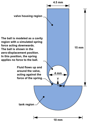
Check valves are commonly used to enforce unidirectional flow of liquids and act as pressure-relieving devices. The check valve for this tutorial contains a ball connected to a spring with a stiffness constant of 300 N/m. The ball is made of steel with a density of 7800 kg/m3 and is represented as a cavity region in the mesh with a diameter of 4 mm. Initially the center of mass of the ball is located at the coordinate point (0, 0.0023, 5e-05); this point is the spring origin, and all forces that interact with the ball are assumed to pass through this point. The tank region, located below the valve housing, is filled with Methanol (CH4O) at 25°C. High pressure from the liquid at the tank opening (6 atm relative pressure) causes the ball to move up, therefore enabling the fluid to escape through the valve to the atmosphere at an absolute pressure of 1 atm. The forces on the ball are: the force due to the spring (not shown in the figure) and the force due to fluid flow. Gravity is neglected here for simplicity. The spring pushes the ball downward to oppose the force of the pressure when the ball is raised above its initial position. The pressure variation causes the ball to oscillate along the Y axis as a result of a dynamic imbalance in the forces. The ball eventually stops oscillating when the forces acting on it are in equilibrium.
In this tutorial the deformation of the ball itself is not modeled; mesh deformation is employed to modify the mesh as the ball moves. A rigid body simulation is used to predict the motion of the ball, and will be based on the forces that act on it.
If this is the first tutorial you are working with, it is important to review the following topics before beginning:
Create a working directory.
Ansys CFX uses a working directory as the default location for loading and saving files for a particular session or project.
Download the
valve_fsi.zipfile here .Unzip
valve_fsi.zipto your working directory.Ensure that the following tutorial input file is in your working directory:
ValveFSI.out
Set the working directory and start CFX-Pre.
For details, see Setting the Working Directory and Starting Ansys CFX in Stand-alone Mode.
This section describes the step-by-step definition of the flow physics in CFX-Pre.
In CFX-Pre, select File > New Case.
Select General and click .
Select File > Save Case As.
Under File name, type
ValveFSI.Click .
Right-click
Meshand select Import Mesh > Other.The Import Mesh dialog box appears.
Configure the following setting(s):
Setting
Value
Files of type
PATRAN Neutral (*out *neu)
File name
ValveFSI.out
Options
> Mesh Units
mm [a]
Click Open.
Right-click
Analysis Typein the Outline tree view and select Edit.Configure the following setting(s):
Tab
Setting
Value
Basic Settings
Analysis Type
> Option
Transient
Analysis Type
> Time Duration
> Option
Total Time
Analysis Type
> Time Duration
> Total Time
7.5e-3 [s]
Analysis Type
> Time Steps
> Option
Timesteps
Analysis Type
> Time Steps
> Timesteps
5.0e-5 [s]
Analysis Type
> Initial Time
> Option
Automatic with Value
Analysis Type
> Initial Time
> Time
0 [s]
Click .
Note: You may ignore the physics validation message regarding the lack of definition of transient results files. You will set up the transient results files later.
In this section you will create the fluid domain, define the fluid and enable mesh motion.
If
Default Domaindoes not currently appear under Flow Analysis 1 in the Outline tree,edit
Case Options>Generalin the Outline tree view and ensure that Automatic Default Domain is turned on and click .In the tree view, right-click
Default Domainand select Edit.Configure the following setting(s):
Tab
Setting
Value
Basic Settings
Location and Type
> Location
CV3D REGION, CV3D SUB [a]
Location and Type
> Domain Type
Fluid Domain
Fluid and Particle Definitions
Fluid 1
Fluid and Particle Definitions
> Fluid 1
> Material
Methanol CH4O [b]
Domain Models
> Pressure
> Reference Pressure
1 [atm]
Domain Models
> Mesh Deformation
> Option
Regions of Motion Specified [c]
Domain Models
> Mesh Deformation
> Displacement Rel. To
Previous Mesh
Domain Models
> Mesh Deformation
> Mesh Motion Model
> Option
Domain Models
> Mesh Deformation
> Mesh Motion Model
> Mesh Stiffness
> Option
Increase near Small Volumes
Domain Models
> Mesh Deformation
> Mesh Motion Model
> Mesh Stiffness
> Model Exponent
1[f]
Domain Models
> Mesh Deformation
> Mesh Motion Model
> Mesh Stiffness
> Reference Volume
> Option
Mean Control Volume
Fluid Models Heat Transfer
> Option
Isothermal
Heat Transfer
> Fluid Temperature
25 [C]
Turbulence
> Option
k-Epsilon
Click the Multi-select from extended list icon
 to open the Selection
Dialog dialog box, then hold the Ctrl key
while selecting both
to open the Selection
Dialog dialog box, then hold the Ctrl key
while selecting both CV3D REGIONandCV3D SUBfrom this list. Click .To make Methanol an available option:
Click the Select from extended list icon
to open the Material dialog box.Click the Import Library Data icon
 to open the Select Library Data to
Import dialog box.
to open the Select Library Data to
Import dialog box. In that dialog box, expand
Constant Property
Liquids
in the tree, selectMethanol CH4Oand click .Select
Methanol CH4Oin the Material dialog box and click .
The
Regions of Motion Specifiedoption permits boundaries and subdomains to move, and makes mesh motion settings available.To see the additional mesh motion settings, you may need to click Roll Down
 located beside Mesh Motion Model.
The Displacement Diffusion model for mesh motion attempts to preserve the relative mesh distribution of the initial mesh.
An exponent value of 1 is chosen in order to limit the distortion of the coarse mesh. If a finer mesh were used, the default value of 2 would most likely be appropriate.
Click .
In this section, a secondary coordinate system will be created to define the center of mass of the ball. This secondary coordinate system will be used to define certain parameters of the rigid body in the next section.
In the Outline tree view, right-click Coordinate Frames and select Insert > Coordinate Frame.
Set the name to
Coord 1and click .Configure the following setting(s):
Tab
Setting
Value
Basic Settings
Option
Axis Points
Origin
(0, 0.0023, 5e-05)
Z Axis Point
(0, 0.0023, 1)
X-Z Plane Pt
(1, 0.0023, 0)
Select .
A rigid body is a non-deformable object described by physical parameters: mass, center of mass, moment of inertia, initial velocities and accelerations, and orientation. The rigid body solver uses the interacting forces between the fluid and the rigid body and calculates the motion of the rigid body based upon the defined physical parameters. The rigid body may have up to six degrees of freedom (three translational and three rotational). You may also specify external forces and torques acting on the rigid body.
In this section, you will define a rigid body with 1 degree of freedom, translation in the Y direction. The rigid body definition will be applied to the wall boundary of the ball to define its motion. Further, you will specify an external spring force by defining a spring constant and the initial origin of the spring; in this simulation the origin is the center of mass of the ball. The force caused by the tank pressure will cause an upward translation and the defined external spring force will resist this translation.
In the Outline tree view, right-click Flow Analysis 1 and select Insert > Rigid Body.
Set the name to
rigidBalland click .Configure the following setting(s):
Tab
Setting
Value
Basic Settings
Mass
9.802e-6 [kg]
Location
BALL
Coordinate Frame
Coord 1
Mass Moment of Inertia
> XX Component
0 [kg m^2] [a]
Mass Moment of Inertia
> YY Component
0 [kg m^2]
Mass Moment of Inertia
> ZZ Component
0 [kg m^2]
Mass Moment of Inertia
> XY Component
0 [kg m^2]
Mass Moment of Inertia
> XZ Component
0 [kg m^2]
Mass Moment of Inertia
> YZ Component
0 [kg m^2]
Dynamics
External Force Definitions
Create a new external force named
Spring Force[b].External Force Definitions
> Spring Force
> Option
Spring
External Force Definitions
> Spring Force
> Equilibrium Position
> X Component
0 [m]
External Force Definitions
> Spring Force
> Equilibrium Position
> Y Component
0 [m]
External Force Definitions
> Spring Force
> Equilibrium Position
> Z Component
0 [m]
External Force Definitions
> Spring Force
> Linear Spring Constant
> X Component
0 [N m^-1]
External Force Definitions
> Spring Force
> Linear Spring Constant
> Y Component
300 [N m^-1]
External Force Definitions
> Spring Force
> Linear Spring Constant
> Z Component
0 [N m^-1]
Degrees of Freedom
> Translational Degrees of Freedom
> Option
Y axis
Degrees of Freedom
> Rotational Degrees of Freedom
> Option
None
Click .
Select Insert > Subdomain from the main menu or click Subdomain
 .
.Set the subdomain name to
Tankand click .Configure the following setting(s):
Tab
Setting
Value
Basic Settings
Location
CV3D SUB
Mesh Motion
Mesh Motion
> Option
Stationary [a]
Click .
In the following subsections, you will create the required boundary conditions, specifying the appropriate mesh motion option for each.
In this tutorial, mesh motion specifications are applied to
two and three dimensional regions of the domain. For example, the Ball boundary specifies the mesh motion in the form of
the rigid body solution. However, mesh motion specifications are also
used in this tutorial to help ensure that the mesh does not fold,
as set for the Tank subdomain earlier in the
tutorial, and the TankOpen boundary below. Two
regions, VALVE HIGHX and VALVE LOWX, remain at the default boundary condition: smooth, no slip walls
and no mesh motion (stationary).
Create a new boundary named
Ball.Configure the following setting(s):
Tab
Setting
Value
Basic Settings
Boundary Type
Wall
Location
BALL
Boundary Details
Mesh Motion
> Option
Rigid Body Solution
Mesh Motion
> Rigid Body
rigidBall
Mass And Momentum
> Option
No Slip Wall
Mass And Momentum
> Wall Vel. Rel. To
Mesh Motion
Click .
Because a 2D representation of the flow field is being modeled (using a 3D mesh, one element thick in the Z direction), you must create symmetry boundaries on the low and high Z 2D regions of the mesh.
Create a new boundary named
Sym.Configure the following setting(s):
Tab
Setting
Value
Basic Settings
Boundary Type
Symmetry
Location
SYMP1, SYMP2 [a]
Boundary Details
Mesh Motion
> Option
Unspecified
Click .
Create a new boundary named
ValveVertWalls.Configure the following setting(s):
Tab
Setting
Value
Basic Settings
Boundary Type
Wall
Location
VPIPE HIGHX, VPIPE LOWX [a]
Boundary Details
Mesh Motion
> Option
Unspecified [b]
Mass And Momentum
> Option
No Slip Wall
Mass And Momentum
> Wall Vel. Rel. To
Boundary Frame
Hold the Ctrl key while selecting both
VPIPE HIGHXandVPIPE LOWXfrom the list.The
Unspecifiedsetting allows the mesh nodes to move freely. The motion of the mesh points on this boundary will be strongly influenced by the motion of the ball. Because the ball moves vertically, the surrounding mesh nodes should also move vertically, at a similar rate to the ball. This mesh motion specification helps to preserve the quality of the mesh on the upper surface of the ball.
Click .
Create a new boundary named
TankOpen.Configure the following setting(s):
Tab
Setting
Value
Basic Settings
Boundary Type
Opening
Location
BOTTOM
Boundary Details
Mesh Motion
> Option
Stationary [a]
Mass And Momentum
> Option
Entrainment
Mass And Momentum
> Relative Pressure
6 [atm] [b]
Turbulence
> Option
Zero Gradient
The stationary option for the tank opening prevents the mesh nodes on this boundary from moving. If the tank opening had unspecified mesh motion, these mesh nodes would move vertically and separate from the non-vertical parts of the boundary.
As defined in the problem description. Note the units for this setting.
Click .
Create a new boundary named
ValveOpen.Configure the following setting(s):
Click .
Note: Opening boundary types are used to enable the flow to leave and reenter the domain. This behavior is expected due to the oscillatory motion of the ball and due to the potentially large region of flow recirculation that may occur downstream from the ball.
Because a transient simulation is being modeled, initial values are required for all variables.
Click Global Initialization
 .
.Configure the following setting(s):
Tab
Setting
Value
Global Settings
Initial Conditions
> Cartesian Velocity Components
> U
0 [m s^-1]
Initial Conditions
> Cartesian Velocity Components
> V
0.1 [m s^-1] [a]
Initial Conditions
> Cartesian Velocity Components
> W
0 [m s^-1]
Initial Conditions
> Static Pressure
> Relative Pressure
0 [Pa]
Initial Conditions
> Turbulence
> Option
Medium (Intensity = 5%)
Click .
In this section you will edit the solver control settings to promote a quicker solution time and to enable the frequency of when the rigid body solver is run.
Click Solver Control
 .
.Configure the following setting(s):
Tab
Setting
Value
Basic Settings
Transient Scheme
> Option
Second Order Backward Euler
Convergence Control
> Max. Coeff. Loops
5
Rigid Body Control
Rigid Body Control
(Selected)
Rigid Body Control
> Rigid Body Solver Coupling Control
> Update Frequency
Every Coefficient Loop [a]
Click .
This step sets up transient results files to be written at set intervals.
Click Output Control
 .
.Click the Trn Results tab.
In the Transient Results tree view, click Add new item
 , set Name to
 Transient Results 1, and click OK.Configure the following setting(s) of
Transient Results 1:Setting
Value
Option
Selected Variables
Output Variables List
Pressure, Velocity
Output Variable Operators
(Selected)
Output Variable Operators
> Output Variable Operators
All [a]
Output Frequency
> Option
Time Interval
Output Frequency
> Time Interval
5.0e-5 [s]
Click the Monitor tab.
Select Monitor Objects.
Under Monitor Points and Expressions:
Click Add new item
.Set Name to
Ball Displacementand click .Set Option to
Expression.Set Expression Value to
rbstate(Position Y)@rigidBall.
Click .

When CFX-Pre has shut down and the CFX-Solver Manager has started, obtain a solution to the CFD problem by following the instructions below.
Ensure that the Define Run dialog box is displayed.
Solver Input File should be set to
ValveFSI.def.Click Start Run.
CFX-Solver runs and attempts to obtain a solution. This can take a long time depending on your system.
Note: You can ignore the warning message indicating a negative sector volume in your mesh. This occurs as a result of large deformations in the mesh and will not significantly affect the results for this case.
While CFX-Solver Manager is running, you can check the progress of the monitor point you created in CFX-Pre by clicking the
User Pointstab in CFX-Solver Manager. The graph shows the Y position of the center of mass of the ball (in the global coordinate frame). Notice that the ball has a sinusoidal motion that diminishes in amplitude over time and that the maximum displacement of the ball occurs at around time step 17.Select Monitors > Rigid Body > Rigid Body Position from the main menu. The position of the rigid body will be shown in the X, Y and Z directions relative to the global coordinate frame.
Note: This graph is identical to the graph obtained from under the
User Pointstab (although the scale may be different). Normally, creating the monitor point for position is redundant since the rigid body positions are calculated automatically — the monitor point was created in this tutorial to demonstrate therbstatefunction.When a dialog box is displayed at the end of the run, select Post-Process Results.
Click .
In the following subsections, you will create a user location, point and vector plots, and an animation in CFD-Post. You will create an XY plane that lies midway between the two symmetry planes. The plane will be used to show the mesh motion; it will also serve as the location for a vector plot that will be used in the animation.
Right-click a blank area in the viewer and select Predefined Camera > View From +Z.
Select Insert > Location > Plane from the main menu. Accept the default name and click .
Configure the following setting(s):
Tab
Setting
Value
Geometry
Definition
> Method
XY Plane
Definition
> Z
5e-05 [m]
Render
Show Faces
(Cleared)
Show Mesh Lines
(Selected)
Click .
Select Insert > Location > Point from the main menu. Accept the default name and click .
Configure the following setting(s):
Tab
Setting
Value
Geometry
Definition
> Method
XYZ
Point
(0, 0.0003, 0)
Symbol
Symbol
Crosshair
Symbol Size
5
Click to create the point.
This is a reference point for the minimum Y value of the ball at time step 0. However the final time step is currently selected. This will be corrected in the proceeding steps.
Select Insert > Location > Point from the main menu. Accept the default name and click .
Configure the following setting(s):
Tab
Setting
Value
Geometry
Definition
> Method
XYZ
Point
(0, 0.001266, 0)
Symbol
Symbol
Crosshair
Symbol Size
5
Click to create the point.
This is a reference point for the minimum Y value of the ball in the positive Y direction at the time of maximum displacement.
Click Timestep Selector
 and load the results for a few
different time steps, selecting one entry at a time.
and load the results for a few
different time steps, selecting one entry at a time.For example, double-click rows with the step values of 0, 10, 20, 50, and 90 to see the ball in different positions. The mesh deformation will also be visible.
Create a new vector named
Vector 1.Configure the following setting(s):
Tab
Setting
Value
Geometry
Locations
Plane 1
Variable
Velocity
Click to show the vector plot in the 3D Viewer.
You will create an animation showing the velocity in the domain as the ball moves.
Turn off the visibility of
Plane 1to better see the vector plot.Click the Timestep Selector
and load the 1st time step.Click Animate timesteps
 in the Timestep Selector dialog box.
The Animation dialog box appears.
Set Type to Keyframe Animation.
Click New
to create KeyframeNo1.Select
KeyframeNo1, then set # of Frames to149, then press Enter while the cursor is in the # of Frames box.Tip: Be sure to press Enter and confirm that the new number appears in the list before continuing.
Use the Timestep Selector to load the last time step.
In the Animation dialog box, click New
to create KeyframeNo2.Tip: The # of Frames parameter has no effect on the last keyframe, so leave it at the default value.
Ensure that More Animation Options
 is pushed down to show more animation settings.
Select Loop.
Ensure that Repeat forever
 (next to the Repeat setting)
is not selected (not pushed down).
(next to the Repeat setting)
is not selected (not pushed down).Click the Options button to open the Animation Options dialog box.
Configure the following setting(s):
Tab
Setting
Value
Options
Print Options
> Image Size
720 x 480 (NTSC)
Advanced
MPEG Options
> Quality
Custom
MPEG Options
> Variable Bit Rate
(Cleared)
MPEG Options
> Bit Rate
3000000 [a]
Click .
Select Save Movie.
Set Format to
MPEG1.Click Browse
 (next
to Save Movie).
(next
to Save Movie).Set File name to
ValveFSI.mpg.If required, set the path to a different directory.
Click .
The movie file name (including the path) has been set, but the animation has not yet been produced.
Click To Beginning
 .
.This ensures that the animation will begin at the first keyframe.
After the first keyframe has been loaded, click Play the animation
 .
.The MPEG will be created as the animation proceeds.
This will be slow, since results for each time step will be loaded and objects will be created.
To view the movie file, you need to use a viewer that supports the MPEG format.
Note: To explore additional animation options, click the Options button. On the Advanced tab of the Animation Options dialog box, there is a Save Frames As Image Files check box. By selecting this check box, the JPEG or PPM files used to encode each frame of the movie will persist after movie creation; otherwise, they will be deleted.
Close the Animation dialog box when the animation is complete.
When you have finished, close the Timestep Selector dialog box and quit CFD-Post.