


This tutorial includes:
In this tutorial you will learn about:
Selection of material properties from the International Association for the Properties of Water and Steam (IAPWS) database.
Setting property table ranges.
Setting up an equilibrium steam calculation.
Reviewing solution variables particular to the equilibrium solution.
Setting up a non-equilibrium steam calculation.
Postprocessing features special to the non-equilibrium solution.
Reviewing solution variables particular to the non-equilibrium solution.
|
Component |
Feature |
Details |
|---|---|---|
|
CFX-Pre |
User Mode |
Turbo Wizard |
|
Machine Type |
Axial Turbine | |
|
Fluid Type |
Homogeneous Binary Mixture (equilibrium solution) | |
|
Multi-Fluid Model (non-equilibrium solution) | ||
|
Domain Type |
Multiple Domain | |
|
Turbulence Model |
k-Epsilon | |
|
Heat Transfer |
Total Energy (equilibrium solution) | |
|
Fluid Dependent (non-equilibrium solution) | ||
|
Boundary Conditions |
Inlet (subsonic): Total Pressure/Temperature and Mass Fraction(s) (equilibrium solution) | |
|
Inlet (subsonic): Total Pressure/Temperature, Volume Fractions and Droplet Number (non-equilibrium solution) | ||
|
Outlet: Static Pressure | ||
|
Domain Interfaces |
Frozen Rotor | |
|
Periodic | ||
|
Timestep |
Physical Time Scale | |
|
Material Properties |
IAPWS Water Database | |
|
Fluid Pair Models |
Small droplet heat transfer, small droplet phase change (non-equilibrium solution) | |
|
Fluid Models |
Nucleation, small droplet temperature, droplets with phase change (non-equilibrium solution) | |
|
CFD-Post |
Location |
Turbo Surface |
|
Plots |
Contour |
The following tutorial uses an axial turbine to demonstrate setting up and executing equilibrium and non-equilibrium steam calculations using the IAPWS water database for properties.
The full geometry contains 60 stator blades and 113 rotor blades. The following figure shows approximately half of the full geometry. The inflow average velocity is in the order of 100 m/s.
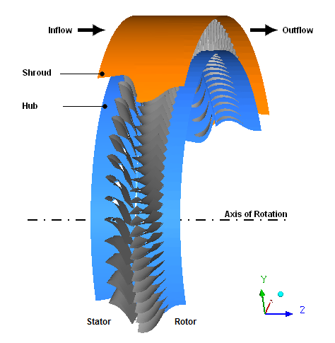
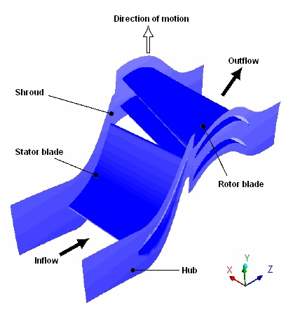
The geometry to be modeled consists of a single stator blade passage and two rotor blade passages. This is an approximation to the full geometry since the ratio of rotor blades to stator blades is close to, but not exactly, 2:1. In the stator blade passage a 6° section is being modeled (360°/60 blades), while in the rotor blade passage, a 6.372° section is being modeled (2*360°/113 blades). This produces a pitch ratio at the interface between the stator and rotor of 0.942. As the flow crosses the interface, it is scaled to enable this type of geometry to be modeled. This results in an approximation of the inflow to the rotor passage. Furthermore, the flow across the interface will not appear continuous due to the scaling applied.
In this example, the rotor rotates at 523.6 rad/s about the Z axis while the stator is stationary. Periodic boundaries are used to enable only a small section of the full geometry to be modeled.
The important problem parameters are:
Total inlet pressure = 0.265 bar
Static outlet pressure = 0.0662 bar
Total inlet temperature = 328.5 K
In this tutorial, you will generate two steady-state solutions: one using a multicomponent fluid consisting of a homogeneous binary mixture of liquid water and water vapor, the other using two separate phases to represent liquid water and water vapor in a non-equilibrium simulation. The solution variables particular to the equilibrium and non-equilibrium solutions will be processed in order to understand the differences between the two solutions.
If this is the first tutorial you are working with, it is important to review the following topics before beginning:
Create a working directory.
Ansys CFX uses a working directory as the default location for loading and saving files for a particular session or project.
Download the
water_vapor.zipfile here .Unzip
water_vapor.zipto your working directory.Ensure that the following tutorial input files are in your working directory:
stator.gtmrotor.grd
Set the working directory and start CFX-Pre.
For details, see Setting the Working Directory and Starting Ansys CFX in Stand-alone Mode.
In this section, you will simulate the equilibrium case where the fluid consists of a homogeneous binary mixture of liquid water and water vapor.
The following sections describe the equilibrium simulation setup in CFX-Pre.
This tutorial uses the Turbomachinery wizard in CFX-Pre. This preprocessing mode is designed to simplify the setup of turbomachinery simulations.
In CFX-Pre, select File > New Case.
Select Turbomachinery and click .
Select File > Save Case As.
Under File name, type
WaterVaporEq.If you are notified the file already exists, click Overwrite.
Click .
In the Basic Settings panel, configure the following setting(s):
Setting
Value
Machine Type
Axial Turbine
Analysis Type
> Type
Steady State
Leave the other settings at their default values.
Click Next.
Create the stator and rotor components as follows:
Right-click a blank area near the Component Definition tree and select Add Component from the shortcut menu.
Create a new component of type
Stationary, namedS1.Beside Mesh > File, click Browse
 .
.The Import Mesh dialog box appears.
Configure the following setting(s):
Setting
Value
File name
stator.gtm [ a ]
Click Open.
Note that when a component is defined, Turbo Mode attempts to configure the Region Information settings, which you can review and manually adjust as necessary.
Create a new component of type
Rotating, namedR1.Set Component Type > Value to 523.6 [radian s^-1].
Beside Mesh > File, click Browse
.The Import Mesh dialog box appears.
Configure the following setting(s):
Setting
Value
File name
rotor.grd [ a ]
Options
> Mesh Units
m
Click Open.
Click Passages and Alignment > Edit.
Configure the following setting(s):
Setting
Value
Passage and Alignment
> Passages/Mesh
> Passages per Mesh
2
Passage and Alignment
> Passages to Model
2
Passage and Alignment
> Passages in 360
113
Click Passages and Alignment > Done.
Click Next.
Note: The components must be ordered as above (stator then rotor)
in order for the interface to be created correctly. The order of the
two components can be changed, if necessary, by right-clicking S1 and selecting Move Component Up.
In this section, you will set properties of the fluid domain
and some solver parameters. Note that initially you will choose the
fluid to be Water Ideal Gas, but later you will
create a new fluid based on the IAPWS database for water and override
this initial setting with it.
In the Physics Definition panel, configure the following setting(s):
Setting
Value
Fluid
Water Ideal Gas
Model Data
> Reference Pressure
0 [atm]
Model Data
> Heat Transfer
Total Energy
Model Data
> Turbulence
k-Epsilon
Inflow/Outflow Boundary Templates
> P-Total Inlet P-Static Outlet
(Selected)
Inflow/Outflow Boundary Templates
> Inflow
> P-Total
0.265 [bar]
Inflow/Outflow Boundary Templates
> Inflow
> T-Total
328.5 [K] [ a ]
Inflow/Outflow Boundary Templates
> Inflow
> Flow Direction
Normal to Boundary
Inflow/Outflow Boundary Templates
> Outflow
> P-Static
0.0662 [bar]
Interface
> Default Type
Frozen Rotor
Solver Parameters
(Selected)
Solver Parameters
> Convergence Control
Physical Timescale
Solver Parameters
> Physical Timescale
0.0005 [s] [ b ]
Click Next.
CFX-Pre will try to create appropriate interfaces using the region names viewed previously in the Region Information section (in the Component Definition setup screen). In this case, you should see that a periodic interface has been generated for both the rotor and the stator. The generated periodic interface can be edited or deleted. Interfaces are required when modeling a small section of the true geometry. An interface is also needed to connect the two components together across the frame change.
Review the various interfaces but do not change them.
Click Next.
CFX-Pre will try to create appropriate boundary conditions using the region names presented previously in the Region Information section. In this case, you should see a list of generated boundary conditions. They can be edited or deleted in the same way as the interface connections that were set up earlier.
Review the various boundary definitions but do not change them.
Click Next.
Set Operation to
Enter General Mode.Click Finish.
After you click Finish, a dialog box appears stating that a Turbo report will not be included in the solver file because you are entering General mode.
Click Yes to continue.
Earlier in the physics definition portion of the Turbomachinery
wizard, you specified Water Ideal Gas as the
fluid in the domain. Here, you will specify a homogeneous binary mixture
to replace it. To create the mixture, you will take two pure fluids
from the IAPWS database for water and combine them. The pure fluids
that will be combined are H2Og, representing
water vapor, and H2Ol, representing liquid water.
The mixture will be named H2Olg.
The present simulations use the published IAPWS-IF97 (International Association for the Properties of Water and Steam - Industrial Formulation 1997) water tables for properties. The published IAPWS-IF97 equations have been implemented in Ansys CFX, enabling you to directly select them for use in your simulations. The present example uses these properties in a tabular format requiring you to specify the range of the properties (such as min/max pressure and temperature bounds) and the number of data points in each table. Note that the IAPWS-IF97 properties have been tested for extrapolation into metastable regions, a fact that will be used for the non-equilibrium calculations that require this kind of state information.
Click Material

Name the new material
H2Og.Enter the following settings for
H2Og:Tab
Setting
Value
Basic Settings
Material Group
IAPWS IF97
Thermodynamic State
(Selected)
Thermodynamic State
> Thermodynamic State
Gas
Material Properties
Thermodynamic Properties
> Table Generation
(Selected)
Thermodynamic Properties
> Table Generation
> Minimum Temperature
(Selected)
Thermodynamic Properties
> Table Generation
> Minimum Temperature
> Min. Temperature
250 [K] [ a ]
Thermodynamic Properties
> Table Generation
> Maximum Temperature
(Selected)
Thermodynamic Properties
> Table Generation
> Maximum Temperature
> Max. Temperature
400 [K]
Thermodynamic Properties
> Table Generation
> Minimum Absolute Pressure
(Selected)
Thermodynamic Properties
> Table Generation
> Minimum Absolute Pressure
> Min. Absolute Pres.
0.01 [bar]
Thermodynamic Properties
> Table Generation
> Maximum Absolute Pressure
(Selected)
Thermodynamic Properties
> Table Generation
> Maximum Absolute Pressure
> Max. Absolute Pres.
0.6 [bar]
Thermodynamic Properties
> Table Generation
> Maximum Points
(Selected)
Thermodynamic Properties
> Table Generation
> Maximum Points
> Maximum Points
100
Click .
In the Outline tree, under
Materials, right-clickH2Ogand select Duplicate.Rename
Copy of H2OgtoH2Ol(using the letter "l" as in "liquid").Open
H2Olfor editing.On the Basic Settings tab, change Thermodynamic State > Thermodynamic State from
GastoLiquid.Click
Create a new material named
H2Olg.Enter the following settings for
H2Olg:Tab
Setting
Value
Basic Settings
Options
Homogeneous Binary Mixture
Material Group
IAPWS IF97
Material 1
H2Og
Material 2
H2Ol
Saturation Properties
Option
IAPWS Library
Table Generation
(Selected)
Table Generation
> Minimum Temperature
(Selected)
Table Generation
> Minimum Temperature
> Min. Temperature
273.15 [K] [ a ]
Table Generation
> Maximum Temperature
(Selected)
Table Generation
> Maximum Temperature
> Max. Temperature
400 [K]
Table Generation
> Minimum Absolute Pressure
(Selected)
Table Generation
> Minimum Absolute Pressure
> Min. Absolute Pres.
0.01 [bar]
Table Generation
> Maximum Absolute Pressure
(Selected)
Table Generation
> Maximum Absolute Pressure
> Max. Absolute Pres.
0.6 [bar]
Table Generation
> Maximum Points
(Selected)
Thermodynamic Properties
> Table Generation
> Maximum Points
> Maximum Points
100
Click .
You now need to update the initial setting for the domain fluid (initially set while in the Turbomachinery wizard) with the new homogeneous binary mixture fluid that you have just created. This mixture (H2Olg) acts as a container fluid identifying two child materials, H2Ol and H2Og, each representing the liquid and vapor properties in the pure fluid system. The equilibrium solution uses the binary mixture fluid, H2Olg, and assumes that equilibrium conditions relate H2Ol and H2Og at all times. In the non-equilibrium solution (in the second part of this tutorial), H2Ol and H2Og are each used separately to define the fluids that are active in the domain; this is a requirement since the equilibrium constraint is no longer applicable in that case.
Open domain
R1for editing.On the Basic Settings tab under Fluid and Particle Definitions, delete any existing items by selecting them and clicking Remove selected item
 .
.Click Add new item
 .
.Set Name to
H2Olgand click OK.Set Fluid and Particle Definitions > H2Olg > Material to
H2Olgand click .On the Fluid Models tab set Component Models > Component > H2Og > Option to
Equilibrium Fraction.Click .
Open
Simulation>Flow Analysis 1>S1>S1 Inletfor editing.On the Boundary Details tab, set Component Details > H2Og > Mass Fraction to
1.0.Click .
Click Global Initialization
 .
.Enter the following settings:
Tab
Setting
Value
Global Settings
Initial Conditions
> Cartesian Velocity Components
> Option
Automatic with Value
Initial Conditions
> Cartesian Velocity Components
> U
0 [m s^-1]
Initial Conditions
> Cartesian Velocity Components
> V
0 [m s^-1]
Initial Conditions
> Cartesian Velocity Components
> W
100 [m s^-1] [ a ]
Initial Conditions
> Static Pressure
> Option
Automatic with Value
Initial Conditions
> Static Pressure
> Relative Pressure
0.2 [bar]
Initial Conditions
> Temperature
> Option
Automatic with Value
Initial Conditions
> Temperature
> Temperature
328.5 [K] [ a ]
Initial Conditions
> Component Details
> H2Og
> Option
Automatic with Value
Initial Conditions
> Component Details
> H2Og
> Mass Fraction
1.0
Click .
Click Define Run
 .
.Configure the following setting(s):
Setting
Value
File name
WaterVaporEq.def
Click .
CFX-Solver Manager automatically starts and, on the Define Run dialog box, Solver Input File is set.
Quit CFX-Pre, saving the simulation (
.cfx) file.
When CFX-Pre has shut down, and CFX-Solver Manager has started, obtain a solution to the CFD problem by following the instructions below.
In CFX-Solver Manager, click Start Run.
At the end of the run, on the completion message that appears, select Post-Process Results.
If using stand-alone mode, select Shut down CFX-Solver Manager.
Click OK.
The equilibrium case produces solution variables unique to these model settings. The most important ones are static pressure, mass fraction and temperature, which will be briefly described here.
When CFD-Post starts, the Domain Selector dialog box might appear. If it does, ensure that both the R1 and S1 domains are selected, then click OK to load the results from these domains.
Click the Turbo tab.
The Turbo Initialization dialog box is displayed, and asks you whether you want to auto-initialize all components. Click Yes.
The Turbo tree view shows the two components in domains
R1andS1. In this case, the initialization works without problems. If there were any problems initializing a component, this would be indicated in the tree view.Note: If you do not see the Turbo Initialization dialog box, or as an alternative to using that dialog box, you can initialize all components by clicking the Initialize All Components button, which is visible initially by default, or after double-clicking the Initialization object in the Turbo tree view.
Make a 2D surface at 50% span to be used as a locator for plots:
On the main menu select Insert > Location > Turbo Surface and name it
Turbo Surface 1.On the Geometry tab, set Method to
Constant
Span
and Value to0.5.Click Apply.
Turn off the visibility of
Turbo Surface 1.
In the equilibrium solution, phase transition occurs the moment saturation conditions are reached in the flow. The amount of moisture ultimately created from phase transition is determined in the following manner.
The static pressure solution field yields the saturation enthalpy
through the function  , available from the IAPWS database. During the solution, if the
predicted mixture static enthalpy,
, available from the IAPWS database. During the solution, if the
predicted mixture static enthalpy,  , falls below
  at any point, the mass fraction of the condensed
phase (also called wetness) can be directly calculated
also based on the IAPWS properties. The degree to which wetness is
generated depends on the amount by which
at any point, the mass fraction of the condensed
phase (also called wetness) can be directly calculated
also based on the IAPWS properties. The degree to which wetness is
generated depends on the amount by which  is less than
  .
.
Note that the mass fraction is predicted at each iteration in the solution, and is used to update other two-phase mixture properties required at each step in the solution. The final results therefore include all of the two-phase influences, but assuming equilibrium conditions. The equilibrium solution mass fraction contour plot will be compared to the non-equilibrium solution one in Viewing the Results Using CFD-Post.
In the next step, you are asked to create the pressure and mass fraction contour plots.
Create a static pressure contour plot on
Turbo Surface 1:Create a new contour plot named
Static Pressure.In the details view on the Geometry tab, set Locations to
Turbo Surface 1and Variable toPressure, then click .
Turn off the visibility of
Static Pressurewhen you have finished observing the results.Create a contour plot on
Turbo Surface 1that shows the mass fraction of the liquid phase:Create a new contour plot named
Mass Fraction of Liquid Phase.In the details view on the Geometry tab, set Locations to
Turbo Surface
1
and Variable toH2Ol.Mass Fraction, then click Apply.
Turn off the visibility of Mass Fraction of Liquid Phase when you have finished observing the results.
In the equilibrium solution, the condensed and gas phases share the same temperature and, as a result, predictions of thermodynamic losses are not possible.
In the following step you are asked to view the temperature field in the solution, and note that, due to the equilibrium constraint, it represents conditions for the mixture.
Create a contour plot on
Turbo Surface 1that shows the static temperature.Create a new contour plot named
Static Temperature.In the details view on the Geometry tab, set Locations to
Turbo Surface 1and Variable toTemperature, then click .
Once you have observed the results save the state and exit CFD-Post.
The non-equilibrium calculation introduces a number of additional
transport equations to the equilibrium solution, namely volume fractions
for each phase and droplet number for all condensing phases. In addition,
energy equations need to be specified for each of the phases in the
solution. The setup of these equations is automated based on model
selections to be described subsequently. Important to the predictions
are interphase heat and mass transfer between the vapor and condensed
phases due to small droplets created by homogeneous nucleation. Selection
of the required phase pair conditions is made easier by provision
of special small droplet models (where small droplet implies droplet
sizes generally below one  ). Phase transition
is initiated based on predicted metastable state (measured by supercooling
level) conditions in the flow in conjunction with a classical homogeneous
nucleation model.
). Phase transition
is initiated based on predicted metastable state (measured by supercooling
level) conditions in the flow in conjunction with a classical homogeneous
nucleation model.
The non-equilibrium solution is therefore closely dependent on the evolving conditions along the flow path leading to phase transition and subsequent strong interaction (by heat/mass transfer) between phases.
Ensure that the following tutorial input file is in your working directory:
WaterVaporEq.cfx
Set the working directory and start CFX-Pre if it is not already running.
For details, see Setting the Working Directory and Starting Ansys CFX in Stand-alone Mode.
Select File > Open Case.
Select the simulation file
WaterVaporEq.cfx.Click Open.
Select File > Save Case As.
Change the name to
WaterVaporNonEq.cfx.Click .
The non-equilibrium case is different from the equilibrium case in that the creation of the second phase (that is, the liquid water) is based on vapor supercooling in conjunction with fluid expansion rate and a nucleation model. The location where the phase transition happens is not specified, but evolves as part of the solution.
In this section, you will specify a nucleation model for the phase that is considered condensable.
You will also set the droplet number and volume fraction of the condensable phase to zero at the inlet. The condensable phase will appear within the domain by homogeneous nucleation. If this case were to involve wetness at the inlet, you would have a choice of specifying either droplet number or droplet diameter as a boundary along with the volume fraction.
Open domain
R1.On the Basic Settings tab under Fluid and Particle Definitions, delete any existing items by selecting them and clicking Remove selected item
.Create two new materials named
H2OgandH2Olby using the Add new item icon.Configure the following setting(s) of domain
R1:Tab
Setting
Value
Basic Settings
Fluid and Particle Definitions
H2Og
Fluid and Particle Definitions
> H2Og
> Material
H2Og
Fluid and Particle Definitions
> H2Og
> Morphology
> Option
Continuous Fluid
Fluid and Particle Definitions
H2Ol
Fluid and Particle Definitions
> H2Ol
> Material
H2Ol
Fluid and Particle Definitions
> H2Ol
> Morphology
> Option
Droplets (Phase Change)
Fluid Models
Multiphase
> Homogeneous Model
(Selected)
Heat Transfer
> Homogeneous Model
(Cleared)
Heat Transfer
> Option
Fluid Dependent
Fluid Specific Models
Fluid
H2Og
Fluid
> H2Og
> Heat Transfer Model
> Option
Total Energy
Fluid
H2Ol
Fluid
> H2Ol
> Heat Transfer Model
> Option
Small Droplet Temperature
Fluid
> H2Ol
> Nucleation Model
(Selected)
Fluid
> H2Ol
> Nucleation Model
> Option
Homogeneous
Fluid
> H2Ol
> Nucleation Model
> Nucleation Bulk Tension Factor [ a ]
(Selected)
Fluid
> H2Ol
> Nucleation Model
> Nucleation Bulk Tension Factor
> Nucleation Bulk Tension
1.0
Fluid Pair Models
Fluid Pair
H2Og | H2Ol
Fluid Pair
> H2Og | H2Ol
> Interphase Transfer
> Option
Particle Model
Fluid Pair
> H2Og | H2Ol
> Mass Transfer
> Option
Phase Change
Fluid Pair
> H2Og | H2Ol
> Mass Transfer
> Phase Change Model
> Option
Small Droplets
Fluid Pair
> H2Og | H2Ol
> Heat Transfer
> Option
Small Droplets
The Nucleation Bulk Tension Factor scales the bulk surface tension values used in the nucleation model. Classical nucleation models are very sensitive to the bulk surface tension, and only slight adjustments will modify the nucleation rate quite significantly. It is common practice in CFD simulations to alter the bulk surface tension values slightly in order to bring results in-line with experiment. Studies suggest that with the IAPWS database and conditions less than 1 bar, a Nucleation Bulk Tension Factor of 1.0 is the best first setting.
Note: The small droplet setting for H2Ol heat transfer implies that the temperature is algebraically determined as a function of the droplet diameter, which in turn is calculated from other solution variables such as H2Ol volume fraction and droplet number.
Click .
Apply the same settings to domain
S1.Most of the settings will have been already copied from domain
R1to domainS1, however the nucleation model settings must be set explicitly.Open
S1 Inletand enter the following settings:Tab
Setting
Value
Boundary Details
Heat Transfer
> Option
Fluid Dependent
Fluid Values
Boundary Conditions
H2Og
Boundary Conditions
> H2Og
> Heat Transfer
> Option
Total Temperature
Boundary Conditions
> H2Og
> Heat Transfer
> Total Temperature
328.5 [K]
Boundary Conditions
> H2Og
> Volume Fraction
> Option
Value
Boundary Conditions
> H2Og
> Volume Fraction
> Volume Fraction
1.0
Boundary Conditions
H2Ol
Boundary Conditions
> H2Ol
> Volume Fraction
> Option
Value
Boundary Conditions
> H2Ol
> Volume Fraction
> Volume Fraction
0
Boundary Conditions
> H2Ol
> Droplet Number
> Option
Specified Number [ a ]
Boundary Conditions
> H2Ol
> Droplet Number
> Droplet Number
0 [m^-3]
Click .
Click Solver Control
 .
.On the Basic Settings tab, set Convergence Control > Fluid Timescale Control > Physical Timescale to
5e-005 [s]and click OK.Because the non-equilibrium simulation involves vapor and therefore tends to be unstable, it is recommended that you set the physical timescale to a relatively small value. The value set here was found to be suitable for this simulation by trial and error.
Click Define Run
.Configure the following setting(s):
Setting
Value
File name
WaterVaporNonEq.def
Click .
CFX-Solver Manager automatically starts and, on the Define Run dialog box, Solver Input File is set.
Quit CFX-Pre, saving the simulation (
.cfx) file at your discretion.
The Define Run dialog box will be displayed when CFX-Solver Manager launches. CFX-Solver Input File will already be set to the name of the CFX-Solver input file just written.
Click Start Run.
CFX-Solver runs and attempts to obtain a solution. At the end of the run, a dialog box is displayed stating that the simulation has ended.
Note: You may notice messages in the solver output regarding problems with evaluating material properties. This is a result of the absolute pressure reaching values outside the range of internal material property tables. In this case, the messages are temporary and stop appearing well before convergence. If you encounter a simulation where the messages persist, or you otherwise suspect that the results might be adversely affected, you can change the ranges of internal material property tables by editing the relevant materials in CFX-Pre.
Select Post-Process Results.
If using stand-alone mode, select Shut down CFX-Solver Manager.
Click OK.
The non-equilibrium calculation creates a number of solution variables. The most important ones, which are briefly described in the following section, are supercooling, nucleation rate, droplet number, mass fraction, and particle diameter.
When CFD-Post starts, the Domain Selector dialog box might appear. If it does, ensure that both the R1 and S1 domains are selected, then click OK to load the results from these domains.
Click the Turbo tab.
The Turbo Initialization dialog box is displayed, and asks you whether you want to auto-initialize all components. Click Yes.
The Turbo tree view shows the two components in domains
R1andS1. In this case, the initialization works without problems. If there were any problems initializing a component, this would be indicated in the tree view.Note: If you do not see the Turbo Initialization dialog box, or as an alternative to using that dialog box, you can initialize all components by clicking the Initialize All Components button, which is visible initially by default, or after double-clicking the Initialization object in the Turbo tree view.
Make a 2D surface at 50% span to be used as a locator for plots:
On the main menu select Insert > Location > Turbo Surface and name it
Turbo Surface 1.On the Geometry tab, set Method to
Constant
Span
and Value to0.5.Click Apply.
Turn off the visibility of
Turbo
Surface 1
.
The non-equilibrium solution provides considerable detail on conditions related to phase transition. In particular, the solution tracks the evolution of metastable conditions in the flow through a supercooling variable obtained on the basis of local pressure and gas phase temperature. The supercooling level is the primary variable influencing the nucleation model. The nucleation model provides an estimate of the rate of production of critically sized nuclei that are stable enough to grow in a supercooled vapor flow.
In the next step, you will plot the degree of supercooling, where the supercooling represents the difference between the saturation temperature, set by the local pressure in the flow, and the associated local gas phase temperature. At the inlet, supercooling is often shown as negative, indicating superheated conditions. At equilibrium conditions, no supercooling is allowed since liquid and vapor phases always share the same temperature. Also, critical homogeneous nucleation at pressures below one atmosphere generally involves supercooling levels of up to 35 to 40 K, depending on rate of expansion in the flow.
Create a supercooling contour plot on
Turbo Surface 1.This will display the degree of non-equilibrium conditions in the gas phase prior to homogeneous phase transition.
Create a new contour plot named
Degree of Supercooling.In the details view on the Geometry tab, set Locations to
Turbo Surface 1and Variable toH2Og.Supercoolingthen click Apply.
Turn off the visibility of
Degree of Supercoolingwhen you have finished observing the results.
In the next step, you will plot the nucleation rate to show the level of nucleation attained, along with the droplet number concentration that is present in the flow following nucleation. Note that the nucleation rates reach very high levels, with peak values remaining in the flow for only a short time (that is, as long as supercooled conditions remain). The supercooled droplets released at nucleation grow rapidly, taking mass from the vapor phase and releasing thermal energy, which acts to rapidly reduce vapor supercooling to near zero. This fact removes further significant nucleation and is why the phase transition process is limited to a narrow region in the flow in most cases.
Create a nucleation rate contour plot on
Turbo Surface 1.This will display the nucleation front at the point of maximum supercooling.
Create a new contour plot named
Nucleation Rate.In the details view on the Geometry tab, set Locations to
Turbo Surface 1and Variable toH2Ol.Nucleation Rate.Set Range to
Localand then click .
Turn off the visibility of
Nucleation Ratewhen you have finished observing the results.Create a droplet number contour plot on
Turbo Surface 1.This will display the predicted droplet concentration resulting from phase transition.
Create a new contour plot named
Droplet Number.In the details view on the Geometry tab, set Locations to
Turbo Surface 1and Variable toH2Ol.Droplet Number.Click .
Turn off the visibility of Droplet Number when you have finished observing the results.
In this section, you will plot the mass fraction (or wetness) of the condensed phase. From the mass fraction and droplet number, it is possible to derive a particle diameter, which you will also plot in this section. Notice that the particle diameters appear in the flow at very small sizes, in the range of 5.0E-9 m, but grow rapidly so that, when leaving the nucleation zone, they are approximately an order of magnitude larger. Since the pressure is dropping through the turbine, droplet sizes continue to increase along with the wetness. To emphasize the particle diameters proceeding out of the nucleation zone, you will set the contour range for viewing. In flow regions near walls, where expansion rate is reduced, small amounts of liquid may have droplet diameters that grow to large sizes relative to those coming from the nucleation zone. Without setting the range, these particle diameters near the walls will be emphasized.
Create a contour plot showing the mass fraction of the condensed phase on
Turbo Surface 1.Condensed droplets grow in size and accumulate mass at the expense of the gas phase.
Create a new contour plot named
Mass Fraction of Condensed Phase H2Ol.In the details view on the Geometry tab, set Locations to
Turbo Surface
1
and Variable toH2Ol.Mass Fraction.Click .
Comparing the mass fraction in the non-equilibrium case to the equilibrium solution previously viewed, you can see that phase transition is considerably delayed such that it occurs in the blade passages of the rotor rather than the stator. This is a typical consequence of non-equilibrium flow, and reflects real flow situations.
Turn off the visibility of Mass Fraction of Condensed Phase H2Ol when you have finished observing the results.
Create a particle diameter contour plot on
Turbo Surface 1.The size of the condensed droplets is calculated from the droplet number and volume fraction of the condensed phase.
Create a new contour plot named
Particle Diameter.In the details view on the Geometry tab, set Locations to
Turbo Surface
1
and Variable toH2Ol.Particle Diameter.Set Range to
User Specifiedthen set Min to0 [m]and Max to1e-07 [m].Click .
Turn off the visibility of
Particle Diameterwhen you have finished observing the results.
In a non-equilibrium prediction, the gas phase temperature is different from the condensed phase temperature. The former is determined from a transport equation and the latter from an algebraic relationship relating droplet temperature to its diameter (through a small droplet model already described).
In this section, you will plot the different temperature fields. It should be noted that, for the case of the condensed phase temperature field, before droplets are actually formed, there is no meaningful droplet temperature. At the point droplets are formed by nucleation, their temperature is at the gas phase. Once the droplets have grown in size, their temperature is very close to the saturation temperature. Because the non-equilibrium solution considers the condensed phase temperatures separate from the gas phase, the influence of thermodynamic losses are included in the predictions. This is because it becomes possible to account for heat flow between the vapor and condensed phases as they pass through the domain. Due to this, non-equilibrium efficiency predictions are more accurate than ones obtained using an equilibrium model.
Create a gas phase static temperature contour plot on
Turbo Surface 1:Create a new contour plot named
Gas Phase Static Temperature.In the details view on the Geometry tab, set Locations to
Turbo Surface
1
and Variable toH2Og.Temperature.Click .
Turn off the visibility of Gas Phase Static Temperature when you have finished observing the results.
Create a condensed phase static temperature contour plot on
Turbo Surface 1.Create a new contour plot named
Condensed Phase Static Temperature.In the details view on the Geometry tab, set Locations to
Turbo Surface
1
and Variable toH2Ol.Temperature.Click .
Once you have observed the results, save the state and exit CFD-Post.