


This tutorial includes:
- 28.1. Tutorial Features
- 28.2. Overview of the Problem to Solve
- 28.3. Preparing the Working Directory
- 28.4. Simulating the Coal Combustion without Swirl and without Nitrogen Oxide
- 28.5. Simulating the Coal Combustion with Swirl and without Nitrogen Oxide
- 28.6. Simulating the Coal Combustion with Swirl and with Nitrogen Oxide
In this tutorial you will learn about:
Importing a CCL file in CFX-Pre.
Setting up and using Proximate/Ultimate analysis for hydrocarbon fuels in CFX-Pre.
Viewing the results for nitrogen oxide in CFD-Post.
|
Component |
Feature |
Details |
|---|---|---|
|
CFX-Pre |
User Mode |
General mode |
|
Analysis Type |
Steady State | |
|
Fluid Type |
Reacting Mixture, Hydrocarbon Fuel | |
|
CCL File |
Import | |
|
Domain Type |
Single Domain | |
|
Boundaries |
Coal Inlet | |
|
Air Inlet | ||
|
Outlet | ||
|
No-slip Wall | ||
|
Periodic | ||
|
Symmetry | ||
|
CFD-Post |
Plots |
Particle Tracking |
In this tutorial, you will model coal combustion and radiation in a furnace. Three different coal combustion simulations will be set up:
Coal Combustion with no-swirl burners where there is no release of nitrogen oxide during the burning process.
Coal Combustion with swirl burners where there is no release of nitrogen oxide during the burning process.
Coal Combustion with swirl burners where there is release of nitrogen oxide during the burning process.
The following figure shows half of the full geometry. The coal
furnace has two inlets: Coal Inlet and Air Inlet, and one outlet. The Coal Inlet (see the inner yellow annulus shown in the figure inset) has air
entering at a mass flow rate of 1.624e-3 kg/s and pulverized coal
particles entering at a mass flow rate of 1.015e-3 kg/s. The Air Inlet (see the outer orange annulus shown in the figure
inset) is where heated air enters the coal furnace at a mass flow
rate of 1.035e-2 kg/s. The outlet is located at the opposite end of
the furnace and is at a pressure of 1 atm.
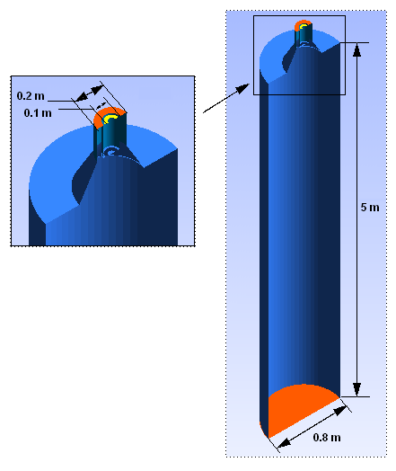
The provided mesh occupies a 5 degree section of an axisymmetric coal furnace. Each simulation will make use of either symmetric or periodic boundaries to model the effects of the remainder of the furnace. In the case of non-swirling flow, a pair of symmetry boundaries is sufficient; in the case of flow with swirl, a periodic boundary with rotational periodicity is required.
The relevant parameters of this problem are:
Coal Inletstatic temperature = 343 KSize distribution for the drops being created by the
Coal Inlet= 12, 38, 62, 88
Air Inletstatic temperature = 573 KOutletaverage static pressure = 0 PaCoal Gunwall fixed temperature = 800 KCoal Inletwall fixed temperature = 343 KAir Inletwall fixed temperature = 573 KFurnace wallfixed temperature = 1400 KO2mass fraction = 0.232Proximate/ultimate analysis data for the coal. Note that proximate/ultimate analysis data is used to characterize the properties of the coal including the content of moisture, volatile, free carbon, and ash, as well as the mass fractions of carbon, hydrogen and oxygen (the major components), sulfur and nitrogen.
The approach for solving this problem is to first import, into CFX-Pre, a CCL file with the proximate/ultimate analysis data for the coal and the required materials and reactions. The first simulation will be without nitrogen oxide or swirl. Only small changes to the boundary conditions will be made to create the second simulation, which has swirl in the flow. After each of the first two simulations, you will use CFD-Post to see the variation of temperature, water mass fraction and radiation intensity. You will examine particle tracks colored by temperature and by ash mass fraction. The last simulation has swirl and also involves the release of nitrogen oxide. Finally, you will use CFD-Post to see the distribution of nitrogen oxide in the third simulation.
If this is the first tutorial you are working with, it is important to review the following topics before beginning:
Create a working directory.
Ansys CFX uses a working directory as the default location for loading and saving files for a particular session or project.
Download the
coal_combustion.zipfile here .Unzip
coal_combustion.zipto your working directory.Ensure that the following tutorial input files are in your working directory:
CoalCombustion.gtmCoalCombustion_Reactions_Materials.ccl
Set the working directory and start CFX-Pre.
For details, see Setting the Working Directory and Starting Ansys CFX in Stand-alone Mode.
You will first create a simulation where there is no release of nitrogen oxide, a hazardous chemical, during the process. Swirl burners will not be used in this simulation.
In CFX-Pre, select File > New Case.
Select General and click .
Select File > Save Case As.
Set File name to
CoalCombustion_nonox.cfx.Click .
Right-click
Meshand select Import Mesh > CFX Mesh.The Import Mesh dialog box appears.
Configure the following setting(s):
Setting
Value
File name
CoalCombustion.gtm
Click Open.
Right-click a blank area in the viewer and select Predefined Camera > Isometric View (Z up) from the shortcut menu.
CFX Command Language (CCL) consists of commands used to carry
out actions in CFX-Pre, CFX-Solver Manager, and CFD-Post. The proximate/ultimate
analysis data for the coal as well as the materials and reactions
required for the combustion simulation will be imported from the CCL
file. You will review, then import, the contents of the CoalCombustion_Reactions_Materials.ccl file.
Note: The physics for a simulation can be saved to a CCL (CFX Command Language) file at any time by selecting File > Export > CCL.
Open
CoalCombustion_Reactions_Materials.cclwith a text editor and take the time to look at the information it contains.The CCL sets up the following reactions:
Fuel Gas OxygenHC Fuel Char FieldHC Fuel DevolatPrompt NO Fuel Gas PDFThermal NO PDF.
The CCL also sets up the following materials:
AshCharFuel GasGas mixtureHC FuelHC Fuel Gas Binary MixtureRaw Combustible
The reactions
Prompt NO Fuel Gas PDFandThermal NO PDFare used only in the third simulation. Other pure substances required for the simulation will be loaded from the standard CFX-Pre materials library.In CFX-Pre, select File > Import > CCL.
The Import CCL dialog box appears.
Under Import Method, select Replace.
This will replace the materials list in the current simulation with the ones in the newly imported CCL.
Under Import Method, select Auto-load materials.
This will load pure materials such as
CO2,H2O,N2,O2, andNO— the materials referenced by the imported mixtures and reactions — from the CFX-Pre materials library.Select
CoalCombustion_Reactions_Materials.ccl(the file you reviewed earlier).Click Open.
Expand the
MaterialsandReactionsbranches underSimulationto make sure that all the materials and reactions described above are present.
Create a new domain named Furnace as
follows:
Right-click
Simulation>Flow Analysis 1in the Outline tree view and click Insert > Domain.Set Name to
Furnace.Click
On the Basic Settings, tab under Fluid and Particle Definitions, delete
Fluid
1
and create a new fluid definition namedGas Mixture.Click Add new item
 and create a new fluid definition
named
and create a new fluid definition
named HC Fuel.Configure the following setting(s):
Tab
Setting
Value
Basic Settings
Location and Type
> Location
B40
Fluid and Particle Definitions
Gas
Mixture
Fluid and Particle Definitions
> Gas Mixture
> Material
Gas Mixture [ a ]
Fluid and Particle Definitions
> Gas Mixture
> Morphology
> Option
Continuous Fluid
Fluid and Particle Definitions
HC Fuel
Fluid and Particle Definitions
> HC Fuel
> Material
HC Fuel [ b ]
Fluid and Particle Definitions
> HC Fuel
> Morphology
> Option
Particle Transport Solid
Fluid and Particle Definitions
> HC Fuel
> Morphology
> Particle Diameter Change
(Selected)
Fluid and Particle Definitions
> HC Fuel
> Morphology
> Particle Diameter Change
> Option
Mass Equivalent[ c ]
Fluid Models
Multiphase
> Multiphase Reactions
(Selected)
Multiphase
> Multiphase Reactions
> Reactions List
HC Fuel Char Field, HC Fuel Devolat
Heat Transfer
> Option
Fluid Dependent
Turbulence
> Option
k-Epsilon
Combustion
> Option
Fluid Dependent
Thermal Radiation
> Option
Fluid Dependent
Fluid Specific Models
Fluid
Gas Mixture
Fluid
> Gas Mixture
> Heat Transfer
> Heat Transfer
> Option
Thermal Energy
Fluid
> Gas Mixture
> Thermal Radiation
> Option
Discrete Transfer
Fluid
> Gas Mixture
> Thermal Radiation
> Number of Rays
(Selected)
Fluid
> Gas Mixture
> Thermal Radiation
> Number of Rays
> Number of Rays
32 [ d ]
Fluid
HC Fuel
Fluid
> HC Fuel
> Heat Transfer
> Heat Transfer
> Option
Particle Temperature
Fluid Pair Models
Fluid Pair
Gas Mixture | HC Fuel
Fluid Pair
> Gas Mixture | HC Fuel
> Particle Coupling
Fully Coupled
Fluid Pair
> Gas Mixture | HC Fuel
> Momentum Transfer
> Drag Force
> Option
Schiller Naumann
Fluid Pair
> Gas Mixture | HC Fuel
> Heat Transfer
> Option
Ranz Marshall
Fluid Pair
> Gas Mixture | HC Fuel
> Thermal Radiation Transfer
> Option
Opaque
Fluid Pair
> Gas Mixture | HC Fuel
> Thermal Radiation Transfer
> Emissivity
1 [ e ]
Fluid Pair
> Gas Mixture | HC Fuel
> Thermal Radiation Transfer
> Particle Coupling
(Selected)
Fluid Pair
> Gas Mixture | HC Fuel
> Thermal Radiation Transfer
> Particle Coupling
> Particle Coupling
Fully Coupled
Click the Ellipsis
 icon to open the Material dialog box, then
select
icon to open the Material dialog box, then
select Gas Mixtureunder theGas Phase Combustionbranch. Click .Click the Ellipsis
icon to open the Material dialog box, then
select HC Fuelunder theParticle Solidsbranch. Click .The use of the
Mass Equivalentoption for the particle diameter is used here for demonstration only. A physically more sensible setting for coal particles, which often stay the same size or get bigger during combustion, would be the use of theSwelling Modeloption with a Swelling Factor of0.0(the default) or larger.Increasing the number of rays to 32 from the default 8, increases the number of rays leaving the bounding surfaces and increases the accuracy of the thermal radiation calculation.
With this setting, the particles are modeled as black bodies.
Click .
In this section you will create boundary conditions for the coal inlet, the air inlet, the outlet, and multiple no-slip walls. You will also create two symmetry-plane boundary conditions for this no-swirl case.
You will create the coal inlet boundary with mass flow rate
and static temperature set consistently with the problem description.
The particle diameter distribution will be set to Discrete
Diameter Distribution to model particles of more than one
specified diameter. Diameter values will be listed as specified in
the problem description. A mass fraction as well as a number fraction
will be specified for each of the diameter entries. The total of mass
fractions and the total of number fractions will sum to unity.
Create a boundary named
Coal Inlet.Configure the following setting(s) of
Coal Inlet:Tab
Setting
Value
Basic Settings
Boundary Type
Inlet
Location
CoalInlet
Boundary Details
Mass and Momentum
> Option
Mass Flow Rate
Mass and Momentum
> Mass Flow Rate
0.001624 [kg s^-1]
Flow Direction
> Option
Normal to Boundary Condition
Heat Transfer
> Option
Static Temperature
Heat Transfer
> Static Temperature
343 [K]
Component Details
O2
Component Details
> O2
> Option
Mass Fraction
Component Details
> O2
> Mass Fraction
0.232
Fluid Values
Boundary Conditions
> HC Fuel
> Particle Behavior
> Define Particle Behavior
(Selected)
Boundary Conditions
> HC Fuel
> Mass and Momentum
> Option
Zero Slip Velocity
Boundary Conditions
> HC Fuel
> Particle Position
> Option
Uniform Injection
Boundary Conditions
> HC Fuel
> Particle Position
> Particle Locations
(Selected)
Boundary Conditions
> HC Fuel
> Particle Position
> Particle Locations
> Particle Locations
Equally Spaced
Boundary Conditions
> HC Fuel
> Particle Position
> Number of Positions
> Option
Direct Specification
Boundary Conditions
> HC Fuel
> Particle Position
> Number of Positions
> Number
200
Boundary Conditions
> HC Fuel
> Particle Mass Flow
> Mass Flow Rate
0.001015 [kg s^-1]
Boundary Conditions
> HC Fuel
> Particle Diameter Distribution
(Selected)
Boundary Conditions
> HC Fuel
> Particle Diameter Distribution
> Option
Discrete
Diameter Distribution
Boundary Conditions
> HC Fuel
> Particle Diameter Distribution
> Diameter List
12, 38, 62, 88 [micron]
Boundary Conditions
> HC Fuel
> Particle Diameter Distribution
> Mass Fraction List
0.18, 0.25, 0.21, 0.36
Boundary Conditions
> HC Fuel
> Particle Diameter Distribution
> Number Fraction List
0.25, 0.25, 0.25, 0.25
Boundary Conditions
> HC Fuel
> Heat Transfer
> Option
Static Temperature
Boundary Conditions
> HC Fuel
> Heat Transfer
> Static Temperature
343 [K]
Click .
Create the air inlet boundary with mass flow rate and static temperature set consistently with the problem description, as follows:
Create a new boundary named
Air Inlet.Configure the following setting(s):
Tab
Setting
Value
Basic Settings
Boundary Type
Inlet
Location
AirInlet
Boundary Details
Mass and Momentum
> Option
Mass Flow Rate
Mass and Momentum
> Mass Flow Rate
0.01035 [kg s^-1]
Flow Direction
> Option
Normal to Boundary Condition
Heat Transfer
> Option
Static Temperature
Heat Transfer
> Static Temperature
573 [K]
Component Details
O2
Component Details
> O2
> Option
Mass Fraction
Component Details
> O2
> Mass Fraction
0.232
Click .
Create the outlet boundary with pressure specified, as follows:
Create a new boundary named
Outlet.Configure the following setting(s):
Tab
Setting
Value
Basic Settings
Boundary Type
Outlet
Location
Outlet
Boundary Details
Mass and Momentum
> Option
Average Static Pressure
Mass and Momentum
> Relative Pressure
0[Pa]
Mass and Momentum
> Pres. Profile Blend
0.05
Click .
Create the Coal Gun Wall boundary with
a fixed temperature as specified in the problem description, as follows:
Create a new boundary named
Coal Gun Wall.Configure the following setting(s):
Tab
Setting
Value
Basic Settings
Boundary Type
Wall
Location
CoalGunWall
Boundary Details
Heat Transfer
> Option
Temperature
Heat Transfer
> Fixed Temperature
800 [K]
Thermal Radiation
> Option
Opaque
Thermal Radiation
> Emissivity
0.6 [ a ]
Thermal Radiation
> Diffuse Fraction
1
Click .
Create the Coal Inlet Wall boundary with
fixed temperature as specified in the problem description, as follows:
Create a new boundary named
Coal Inlet Wall.Configure the following setting(s):
Tab
Setting
Value
Basic Settings
Boundary Type
Wall
Location
CoalInletInnerWall, CoalInletOuterWall [ a ]
Boundary Details
Heat Transfer
> Option
Temperature
Heat Transfer
> Fixed Temperature
343 [K]
Thermal Radiation
> Option
Opaque
Thermal Radiation
> Emissivity
0.6
Thermal Radiation
> Diffuse Fraction
1
Click .
Create the Air Inlet Wall boundary with
fixed temperature as specified in the problem description, as follows:
Create a new boundary named
Air Inlet Wall.Configure the following setting(s):
Tab
Setting
Value
Basic Settings
Boundary Type
Wall
Location
AirInletInnerWall, AirInletOuterWall
Boundary Details
Heat Transfer
> Option
Temperature
Heat Transfer
> Fixed Temperature
573 [K]
Thermal Radiation
> Option
Opaque
Thermal Radiation
> Emissivity
0.6
Thermal Radiation
> Diffuse Fraction
1
Click .
Create the Furnace Wall boundary with a
fixed temperature as specified in the problem description, as follows:
Create a new boundary named
Furnace Wall.Configure the following setting(s):
Tab
Setting
Value
Basic Settings
Boundary Type
Wall
Location
FurnaceFrontWall, FurnaceOuterWall
Boundary Details
Heat Transfer
> Option
Temperature
Heat Transfer
> Fixed Temperature
1400 [K]
Thermal Radiation
> Option
Opaque
Thermal Radiation
> Emissivity
0.6
Thermal Radiation
> Diffuse Fraction
1
Click .
Create a new boundary named
Quarl Wall.Configure the following setting(s):
Tab
Setting
Value
Basic Settings
Boundary Type
Wall
Location
QuarlWall
Boundary Details
Heat Transfer
> Option
Temperature
Heat Transfer
> Fixed Temperature
1200 [K]
Thermal Radiation
> Option
Opaque
Thermal Radiation
> Emissivity
0.6
Thermal Radiation
> Diffuse Fraction
1
Click .
You will use symmetry plane boundaries on the front and back regions of the cavity.
Create a new boundary named
Symmetry Plane 1.Configure the following setting(s):
Tab
Setting
Value
Basic Settings
Boundary Type
Symmetry
Location
PeriodicSide1
Click .
Create a new boundary named
Symmetry Plane 2.Configure the following setting(s):
Tab
Setting
Value
Basic Settings
Boundary Type
Symmetry
Location
PeriodicSide2
Click .
Click Solver Control
 .
.Configure the following setting(s):
Tab
Setting
Value
Basic Settings
Convergence Control
> Max. Iterations
600
Convergence Control
> Fluid Timescale Control
> Timescale Control
Physical Timescale
Convergence Control
> Fluid Timescale Control
> Physical Timescale
0.005 [s] [ a ]
Particle Control
Particle Coupling Control
> First Iteration for Particle Calculation
(Selected)
Particle Coupling Control
> First Iteration for Particle Calculation
> First Iteration
25 [ b ]
Particle Coupling Control
> Iteration Frequency
(Selected)
Particle Coupling Control
> Iteration Frequency
> Iteration Frequency
10 [ c ]
Particle Under Relaxation Factors
(Selected)
Particle Under Relaxation Factors
> Vel. Under Relaxation
0.75
Particle Under Relaxation Factors
> Energy
0.75
Particle Under Relaxation Factors
> Mass
0.75
Particle Ignition
(Selected)
Particle Ignition
> Ignition Temperature
1000 [K]
Particle Source Smoothing
(Selected)
Particle Source Smoothing
> Option
Smooth
Advanced Options
Thermal Radiation Control
(Selected)
Thermal Radiation Control
> Coarsening Control
(Selected)
Thermal Radiation Control
> Coarsening Control
> Target Coarsening Rate
(Selected)
Thermal Radiation Control
> Coarsening Control
> Target Coarsening Rate
> Rate
16 [ d ]
The First Iteration parameter sets the coefficient-loop iteration number at which particles are first tracked; it allows the continuous-phase flow to develop before tracking droplets through the flow. Experience has shown that the value usually has to be increased to 25 from the default of 10.
The Iteration Frequency parameter is the frequency at which particles are injected into the flow after the First Iteration for Particle Calculation iteration number. The iteration frequency allows the continuous phase to settle down between injections because it is affected by sources of momentum, heat, and mass from the droplet phase. Experience has shown that the value usually has to be increased to 10 from the default of 5.
The Target Coarsening Rate parameter controls the size of the radiation element required for calculating Thermal Radiation. Decreasing the size of the element to 16, from the default 64, increases the accuracy of the solution obtained, while increasing the computing time required for the calculations.
Click .
Click Define Run
 .
.Configure the following setting(s):
Setting
Value
File name
CoalCombustion_nonox.def
Click .
CFX-Solver Manager automatically starts and, on the Define Run dialog box, Solver Input File is set.
Quit CFX-Pre, saving the simulation (
.cfx) file.
When CFX-Pre has shut down and the CFX-Solver Manager has started, obtain a solution to the CFD problem by following the instructions below:
Ensure that the Define Run dialog box is displayed.
Solver Input File should be set to
CoalCombustion_nonox.def.Click Start Run.
CFX-Solver runs and attempts to obtain a solution. At the end of the run, a dialog box is displayed stating that the simulation has ended.
Select Post-Process Results.
If using stand-alone mode, select Shut down CFX-Solver Manager.
Click .
In this section, you will make plots showing the variation of
temperature, water mass fraction, and radiation intensity on the Symmetry Plane 1 boundary. You will also color the particle
tracks, which were produced by the solver and included in the results
file, by temperature and by ash mass fraction. The particle tracks
help to illustrate the mean flow behavior in the coal furnace.
Right-click a blank area in the viewer and select Predefined Camera > Isometric View (Z up).
This orients the geometry with the inlets at the top, as shown at the beginning of this tutorial.
Edit
Cases>CoalCombustion_nonox_001>Furnace>Symmetry Plane 1.Configure the following setting(s):
Tab
Setting
Value
Color
Mode
Variable
Variable
Temperature
Render
Show Faces
(Selected)
Lighting
(Cleared) [ a ]
Click .
As expected for a non-swirling case, the flame appears a significant distance away from the burner. The flame is likely unstable, as evidenced by the rate of solver convergence; the next simulation in this tutorial involves swirl, which tends to stabilize the flame, and has much faster solver convergence.
Change the variable used for coloring the plot to H2O.Mass Fraction and click Apply.
From the plot it can be seen that water is produced a significant distance away from the burner, as was the flame in the previous plot. As expected, the mass fraction of water is high where the temperature is high.
Change the variable used for coloring the plot to
Radiation Intensityand click Apply.This plot is directly related to the temperature plot. This result is consistent with radiation being proportional to temperature to the fourth power.
When you are finished, right-click
Symmetry Plane 1in the Outline tree view and select Hide.
Color the existing particle tracks for the solid particles by temperature:
Edit
Cases>CoalCombustion_nonox_001>Res PT for HC Fuel.Configure the following setting(s):
Tab
Setting
Value
Color
Mode
Variable
Variable
HC Fuel.Temperature
Click .
Observing the particle tracks, you can see that coal enters the chamber at a temperature of around 343 K. The temperature of the coal, as it moves away from the inlet, rises as it reacts with the air entering from the inlet. The general location where the temperature of the coal increases rapidly is close to the location where the flame appears to be according to the plots created earlier. Downstream of this location, the temperature of the coal particles begins to drop.
You will now create a simulation where swirl burners are used and where there is no release of nitrogen oxide during the process. Swirl burners inject a fuel axially into the combustion chamber surrounded by an annular flow of oxidant (normally air) that has, upon injection, some tangential momentum. This rotational component, together with the usually divergent geometry of the burner mouth, cause two important effects:
They promote intense mixing between fuel and air, which is important for an efficient and stable combustion, and low emissions.
They originate a recirculation region, just at the burner mouth, which traps hot combustion products and acts as a permanent ignition source, hence promoting the stability of the flame.
Ensure that the following tutorial input file is in your working directory:
CoalCombustion_nonox.cfx
Set the working directory and start CFX-Pre if it is not already running.
For details, see Setting the Working Directory and Starting Ansys CFX in Stand-alone Mode.
Select File > Open Case.
From your working directory, select
CoalCombustion_nonox.cfxand click Open.Select File > Save Case As.
Set File name to
CoalCombustion_nonox_swirl.cfx.Click .
To add swirl to the flow, you will edit the Air
Inlet boundary to change the flow direction specification
from Normal to Boundary Condition to Cylindrical Components. You will also edit the Outlet boundary to change the Pressure Profile
Blend setting from 0.05 to 0; the reason for this change
is explained later. You will also delete the two symmetry plane boundary
conditions and replace them with a periodic domain interface.
Edit
Simulation>Flow Analysis 1>Furnace>Air Inlet.Configure the following setting(s):
Tab
Setting
Value
Boundary Details Flow Direction
> Option
Cylindrical Components
Flow Direction
> Axial Component
0.88
Flow Direction
> Radial Component
0
Flow Direction
> Theta Component
1
Axis Definition
> Rotational Axis
Global Z
Click .
The average pressure boundary condition leaves the pressure profile unspecified while constraining the average pressure to the specified value. In some situations, leaving the profile fully unspecified is too weak and convergence difficulties may result. The 'Pressure Profile Blend' feature works around this by blending between an unspecified pressure profile and a fully specified pressure profile. By default, the pressure profile blend is 5%. For swirling flow, however, imposing any amount of a uniform pressure profile is inconsistent with the radial pressure profile which should naturally develop in response to the fluid rotation, and the pressure profile blend must be set to 0.
Edit
Simulation>Flow Analysis 1>Furnace>Outlet.Configure the following setting(s):
Tab
Setting
Value
Boundary Details
Mass and Momentum
> Option
Average Static Pressure
Mass and Momentum
> Pres. Profile Blend
0
Click .
You will insert a domain interface to connect the Periodic Side 1 and Periodic Side 2 regions.
Create a domain interface named
Periodic.Configure the following setting(s):
Tab
Setting
Value
Basic Settings
Interface Type
Fluid Fluid
Interface Side 1
> Region List
PeriodicSide1
Interface Side 2
> Region List
PeriodicSide2
Interface Models
> Option
Rotational Periodicity
Click .
Click Define Run
.Configure the following setting(s):
Setting
Value
File name
CoalCombustion_nonox_swirl.def
Click .
CFX-Solver Manager automatically starts and, on the Define Run dialog box, Solver Input File is set.
Quit CFX-Pre, saving the simulation (
.cfx) file.
When CFX-Pre has shut down and the CFX-Solver Manager has started, obtain a solution to the CFD problem by following the instructions below.
Ensure that the Define Run dialog box is displayed.
Solver Input File should be set to
CoalCombustion_nonox_swirl.def.Click Start Run.
CFX-Solver runs and attempts to obtain a solution. At the end of the run, a dialog box is displayed stating that the simulation has ended.
Select Post-Process Results.
If using stand-alone mode, select Shut down CFX-Solver Manager.
Click .
In this section, you will make plots showing the variation of
temperature, water mass fraction, and radiation intensity on the Periodic Side 1 boundary. You will also color the existing
particle tracks by temperature and by ash mass fraction.
Right-click a blank area in the viewer and select Predefined Camera > Isometric View (Z up).
Edit
Cases>CoalCombustion_nonox_swirl_001>Furnace>Periodic Side 1.Configure the following setting(s):
Tab
Setting
Value
Color
Mode
Variable
Variable
Temperature
Render
Show Faces
(Selected)
Lighting
(Cleared)
Click .
As expected, the flame appears much closer to the burner than in the previous simulation, which had no swirl. This is due to the fact that the swirl component applied to the air from
Air Inlettends to entrain coal particles and keep them near the burner for longer, therefore helping them to burn.
Change the variable used for coloring the plot to H2O.Mass Fraction and click Apply.
Similar to the no-swirl case, the mass fraction of water with swirl is directly proportional to the temperature of the furnace.
Change the variable used for coloring the plot to
Radiation Intensityand click Apply.When you are finished, right-click
Periodic
Side 1
in the Outline tree view and select Hide.
Edit
Cases>CoalCombustion_nonox_swirl_001>Res PT for HC Fuel.Configure the following setting(s):
Tab
Setting
Value
Color
Mode
Variable
Variable
HC Fuel.Temperature
Click .
You will now create a simulation that involves both swirl and
the release of nitrogen oxide. The CCL file that was previously imported
contains the nitrogen oxide material, NO, and
reactions, Prompt NO Fuel Gas PDF and Thermal NO PDF, required for this combustion simulation.
Nitrogen oxide is calculated as a postprocessing step in the solver.
Ensure that the following tutorial input files are in your working directory:
CoalCombustion_nonox_swirl.cfxCoalCombustion_nonox_swirl_001.res
Set the working directory and start CFX-Pre if it is not already running.
For details, see Setting the Working Directory and Starting Ansys CFX in Stand-alone Mode.
Select File > Open Case.
From your working directory, select
CoalCombustion_nonox_swirl.cfxand click Open.Select File > Save Case As.
Set File name to
CoalCombustion_noxcpp_swirl.cfx.Click .
In this section, you will edit the Furnace domain by adding the new material NO to the
materials list. CFX-Solver requires that you specify enough information
for the mass fraction of NO at each of the system
inlets. In this case, set the NO mass fraction
at the air and coal inlets to zero.
Edit
Simulation>Flow Analysis 1>Furnace.Configure the following setting(s):
Tab
Setting
Value
Fluid Specific Models
Fluid
Gas Mixture
Fluid
> Gas Mixture
> Combustion
> Chemistry Post Processing
(Selected)
Fluid
> Gas Mixture
> Combustion
> Chemistry Post Processing
> Materials List
NO
Fluid
> Gas Mixture
> Combustion
> Chemistry Post Processing
> Reactions List
Prompt NO Fuel Gas PDF,Thermal NO PDF
These settings enable the combustion simulation with nitrogen oxide (NO) as a postprocessing step in the solver. The NO reactions are defined in the same way as any participating reaction but the simulation of the NO reactions is performed after the combustion simulation of the air and coal. With this one-way simulation, the NO will have no effect on the combustion simulation of the air and coal.
Click .
Edit
Simulation>Flow Analysis 1>Furnace>Air Inlet.Configure the following setting(s):
Tab
Setting
Value
Boundary Details
Component Details
NO
Component Details
> NO
> Mass Fraction
0.0
Click .
Edit
Simulation>Flow Analysis 1>Furnace>Coal Inlet.Configure the following setting(s):
Tab
Setting
Value
Boundary Details
Component Details
NO
Component Details
> NO
> Mass Fraction
0.0
Click .
When CFX-Pre has shut down and the CFX-Solver Manager has started, obtain a solution to the CFD problem by following the instructions below.
Ensure that the Define Run dialog box is displayed.
Solver Input File should be set to
CoalCombustion_noxcpp_swirl.def.Under the Initial Values tab, select Initial Values Specification.
Select
CoalCombustion_nonox_swirl_001.resfor the initial values file using the Browse tool.
tool.The fluid solution from the previous case has not changed for this simulation. Loading the results from the previous case as an initial guess eliminates the need for the solver to solve for the fluids solutions again.
Click Start Run.
CFX-Solver runs and attempts to obtain a solution. At the end of the run, a dialog box is displayed stating that the simulation has ended.
Select Post-Process Results.
If using stand-alone mode, select Shut down CFX-Solver Manager.
Click .
In this section, you will make a plot on the Periodic
Side 1 region showing the variation of concentration of
nitrogen oxide through the coal furnace.
Right-click a blank area in the viewer and select Predefined Camera > Isometric View (Z up).
Edit
Cases>CoalCombustion_noxcpp_swirl_001>Furnace>Periodic Side 1.Configure the following setting(s):
Tab
Setting
Value
Color
Mode
Variable
Variable
NO.Mass Fraction
Render
Show Faces
(Selected)
Lighting
(Cleared)
Click .
You can see that NO is produced in the high-temperature region near the inlet. Further downstream, the mass fraction of NO is more uniform.
Quit CFD-Post, saving the state (
.cst) file at your discretion.