


This tutorial includes:
In this tutorial you will learn about:
Importing a CCL file in CFX-Pre.
High-speed multicomponent, multiphase flow with interphase mass transfer.
Model customization using CEL.
Handling mass sources based on species transfer.
Source linearization.
Component | Feature | Details |
|---|---|---|
CFX-Pre | User Mode | General mode |
Domain Type | Single Domain | |
Analysis Type | Steady State | |
Fluid Type | Continuous Fluid | |
Dispersed Fluid | ||
CCL File | Import | |
Boundary Conditions | Inlet Boundary | |
Opening Boundary | ||
Outlet Boundary | ||
Steam Jet Default | ||
Symmetry Boundary | ||
Timestep | Physical Timescale | |
CFD-Post | Plots | Default Locators |
Line Locator | ||
Other | Chart Creation |
This tutorial investigates the simulation of a high-speed steam jet from a pipe. Steam at 373 K leaves the pipe at 341 m s^-1 and contains some liquid water. The surrounding air temperature is 25 °C.
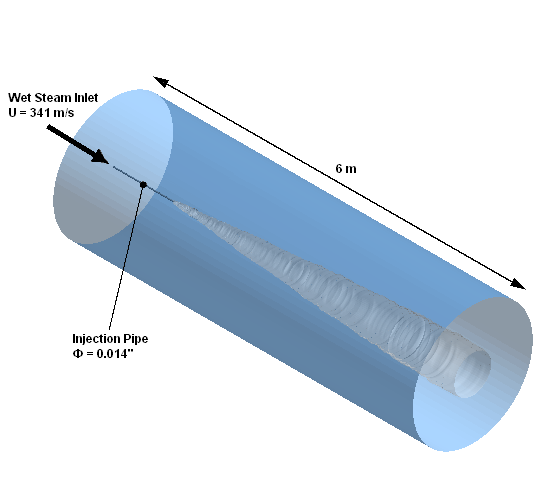
Evaporation and condensation of water are modeled using mass sources and sinks applied to two subdomains; one is used for evaporation and the other is used for condensation. The rate of mass transfer is modeled using Sherwood number-based mass diffusion at the surface of liquid drops.
To take advantage of the symmetrical nature of the domain, a thin slice of the flow field is modeled and symmetry boundaries are used to represent the rest of the flow field. An opening boundary is used around the outside edges of the domain; the flow direction is restricted to be normal to this boundary in order to provide sufficient constraints on the flow solution.
It is strongly recommended that you complete the previous tutorials before trying this one. However, if this is the first tutorial you are working with, it is important to review the following topics before beginning:
Create a working directory.
Ansys CFX uses a working directory as the default location for loading and saving files for a particular session or project.
Download the
steam_jet.zipfile here .Unzip
steam_jet.zipto your working directory.Ensure that the following tutorial input files are in your working directory:
steam_jet.gtmsteam_jet_expressions.cclsteam_jet_additional_variables.ccl
Set the working directory and start CFX-Pre.
For details, see Setting the Working Directory and Starting Ansys CFX in Stand-alone Mode.
This section describes the step-by-step definition of the flow physics in CFX-Pre for a steady-state simulation.
In CFX-Pre, select File > New Case.
Select General and click .
Select File > Save Case As.
Set File name to
SteamJet.cfx.Click .
Right-click
Meshand select Import Mesh > CFX Mesh.The Import Mesh dialog box appears.
Configure the following setting(s):
Setting
Value
File name
steam_jet.gtm
Click Open.
CFX Command Language (CCL) consists of commands used to
carry out actions in CFX-Pre, CFX-Solver Manager, and CFD-Post. Expressions
and Additional Variables required for the steam jet simulation will
be imported from CCL files. This section outlines the steps to analyze steam_jet_expressions.ccl and steam_jet_additional_variables.ccl, and then import them into the simulation.
Note: The physics for a case can be saved to a CCL (CFX Command Language) file at any time by selecting File > Export > CCL.
Select CCL files from your working directory, and open them one at a time with a text editor and take the time to look at the information they contain. The information contained in the CCL files is outlined below:
The CCL file
steam_jet_expressions.cclcreates expressions required for setting up the following data:Liquid/gas interface
Interphase diffusive transport coefficient
Heats of vaporization
Liquid-gas mass transfer rate for water [1]
Local false step linearization of the interphase mass transfer (IPMT).
The CCL file
steam_jet_additional_variables.cclcreates the following Additional Variables:Pressure linearization coefficient
PCoefWater IPMT flux liquid-to-gas
WaFluxLGWater IPMT flux gas-to-liquid
WaFluxGLLocal IPMT false timestep
FalseDtSaturation temperature
SatTempSaturation pressure
SatPresLatent heat at saturation
SatLHeat
These variables are recognizable by CFD-Post to enable plotting and further analysis during postprocessing.
Select File > Import > CCL
The Import CCL dialog box appears.
Under Import Method, select Append. This option appends the changes to the existing case.
Note: The Replace option is useful if you have defined the physics and want to update or replace the existing physics using the newly imported CCL.
From your working directory, select
steam_jet_expressions.ccl.Click Open. The CCL is now loaded as indicated by the status bar in the bottom right corner of the window. After a short pause, the CCL and the Outline tree view will be updated.
Repeat steps 2 to 5 to import
steam_jet_additional_variables.ccl.In the Outline tree view, expand the
Additional VariablesandExpressionsbranches underSimulation>Expressions, Functions and Variablesto confirm that new objects have been added after importing the CCL files.
The characteristics of this case do not change as a function of time, and therefore a steady-state analysis is appropriate.
Right-click
Analysis Typein the Outline tree view and select Edit.Configure the following setting(s):
Tab
Setting
Value
Basic Settings
Analysis Type
> Option
Steady State
Click .
In addition to providing template fluids, CFX allows you to create custom fluids for use in all your CFX models. A custom fluid may be defined as a pure substance, but may also be defined as a mixture, consisting of a number of transported fluid components. This type of fluid model is useful for applications involving mixtures, reactions, and combustion.
In order to define custom fluids, CFX-Pre provides the Material details view. This tool allows you to define your own fluids as pure substances, fixed composition mixtures or variable composition mixtures using a range of template property sets defined for common materials.
The steam jet application requires two fluids: a variable-composition
mixture containing the materials Steam3v (which
is dry steam) and Air Ideal Gas; a fixed-composition
mixture containing only the material Steam3l (which
is liquid water). In a variable composition mixture, the proportion
of each component material will change throughout the simulation;
while in a fixed composition mixture, the proportion of each component
material is fixed.
You are first going to load some of the materials that take
part in the process (Steam3v, Steam3l). The only other material that takes part in the process, Air Ideal Gas, is already loaded.
Load the materials Steam3v and Steam3l from the CFX-Pre Materials Library by loading Steam3vl.
In the Outline tree view, right-click
Simulation>Materialsand select Import Library Data.The Select Library Data to Import dialog box appears.
Click the browse button
 next to File to Import.
 The Import CCL dialog box appears. If the dialog box opens behind any existing windows, reposition it so that it is completely visible in order to complete the next step.
Under Import Method, select Append. This option appends the CCL changes to the existing case.
Select
MATERIALS-iapws.cclfrom theetc/materials-extradirectory and click Open.In the Select Library Data to Import dialog box, expand
Wet Steamand selectSteam3vl.Click .
In the Outline tree view, expand
Simulation>Materialsto confirm thatSteam3vandSteam3lhave been added to the list.
In the next sections you will create the variable-composition mixture and the fixed-composition mixture.
Create a new material named Gas mixture that will be composed of Air Ideal Gas and Steam3v. This material will be injected into the gas inlet
during the steady-state simulation.
Create a new material named
Gas mixture.Configure the following setting(s):
Tab
Setting
Value
Basic Settings
Option
Variable Composition Mixture
Materials List
Air Ideal Gas, Steam3v [a]
Click .
Create a new material named Liquid mixture that will be composed of Steam3l.
Create a new material named
Liquid mixture.Configure the following setting(s):
Tab
Setting
Value
Basic Settings
Option
Fixed Composition Mixture
Materials List
Steam3l
Child Materials
> Steam3l
> Mass Fraction
1.0
Click .
This section outlines the steps to create a new domain Steam Jet.
Select Insert > Domain from the menu bar, or click Domain
 .
.In the Insert Domain dialog box, set the name to
Steam Jetand click .On the Basic Settings tab, configure the following setting(s) under Location and Type:
Setting
Value
Location
B26
Domain Type
Fluid Domain
Coordinate Frame
Coord 0
On the Basic Settings tab, delete any existing items under Fluid and Particle Definitions by selecting them and clicking Remove selected item
 .
.Under Fluid and Particle Definitions, create two fluid definitions named
GasandLiquidby using the Add new item icon.
icon.The new fluids named
GasandLiquidappear under Fluid and Particle Definitions.On the Basic Settings tab, configure the following setting(s) under Fluid and Particle Definitions:
Setting
Value
(List Box)
Gas
Gas
> Material
Gas mixture
Gas
> Morphology
> Option
Continuous Fluid
(List Box)
Liquid
Liquid
> Material
Liquid mixture
Liquid
> Morphology
> Option
Dispersed Fluid
Liquid
> Morphology
> Mean Diameter
liqLength [a]
On the Fluid Models tab, configure the following setting(s):
Setting
Value
Heat Transfer
> Option
Fluid Dependent
Turbulence
> Option
Fluid Dependent
Combustion
> Option
None
Thermal Radiation
> Option
None
On the Fluid Models tab under Additional Variable Models > Additional Variable, select
FalseDtand select the FalseDt check box.Make sure that Additional Variable Models > Additional Variable > FalseDt > Option is set to
Fluid Dependent.Repeat the previous two steps for the rest of the Additional Variables (PCoef, SatLheat, SatPres, SatTemp, WaFluxGL, WaFluxLG).
On the Fluid Specific Models tab, select
Gasin the list box, then configure the following setting(s):Setting
Value
Heat Transfer Model
> Option
Total Energy
Turbulence
> Option
k-Epsilon
Turbulence
> Wall Function
> Wall Function
Scalable
Component Models
> Component
Air Ideal Gas
Component Models
> Component
> Air Ideal Gas
> Option
Constraint
Component Models
> Component
Steam3v
Component Models
> Component
> Steam3v
> Option
Transport Equation
Component Models
> Component
> Steam3v
> Kinematic Diffusivity
(Selected)
Component Models
> Component
> Steam3v
> Kinematic Diffusivity
> Kinematic Diffusivity
KinDiff
Additional Variable Models
PCoef
Additional Variable Models
> PCoef
(Selected)
Additional Variable Models
> PCoef
> Add. Var. Value
dFLUXwadp
On the Fluid Specific Models tab, select
Liquidin the list box, then configure the following setting(s):Setting
Value
Heat Transfer Model
> Option
Total Energy
Turbulence
> Option
Dispersed Phase Zero Equation
Under Additional Variable Models (for Liquid), select
FalseDtin the list box, then configure the following setting(s):Setting
Value
FalseDt
(Selected)
FalseDt
> Add. Var. Value
DtFalseMf
Repeat the previous step for the rest of the Additional Variables (PCoef, SatLheat, SatPres, SatTemp, WaFluxGL, WaFluxLG) using the following values:
Additional Variable
Expression
PCoef
dFLUXwadp
SatLheat
HtVapwa
SatPres
VpWat
SatTemp
SatT
WaFluxGL
FLUXwa1
WaFluxLG
FLUXwa2
On the Fluid Pair Models tab, select
Gas | Liquidin the list box, then configure the following setting(s):Setting
Value
Surface Tension Coefficient
(Selected)
Surface Tension Coefficient
> Surf. Tension Coeff.
srfTenCoef
Interphase Transfer
> Option
Particle Model
Momentum Transfer
> Drag Force
> Option
Schiller Naumann
Turbulence Transfer
> Option
None
Mass Transfer
> Option
None
Heat Transfer
> Option
Ranz Marshall
Click .

To model evaporation and condensation, mass sources and sinks
are defined for the materials Steam3v and Steam3l, according to the expressions imported earlier.
In the next two sections you will set up two subdomains; one is used
for evaporation and the other is used for condensation.
This section outlines the steps to create the subdomain GastoLiq. This subdomain will be defined in a manner consistent
with the process of condensation.
Create a subdomain named
GastoLiq.On the Basic Settings tab, configure the following setting(s):
Setting
Value
Location
B26
Coordinate Frame
Coord 0
On the Fluid Sources tab, select
Gasin the list box, then select the Gas check box and configure the following setting(s):Setting
Value
Equation Sources
Continuity
Equation Sources
> Continuity
(Selected)
Equation Sources
> Continuity
> Option
Fluid Mass Source
Equation Sources
> Continuity
> Source
-Liquid.WaFluxGL
Equation Sources
> Continuity
> MCF/Energy Sink Option
(Selected)
Equation Sources
> Continuity
> MCF/Energy Sink Option
> Sink Option
Spec. Mass Frac. and Loc. Temp.
Equation Sources
> Continuity
> Mass Source Volume Fraction Coefficient
(Selected)
Equation Sources
> Continuity
> Mass Source Volume Fraction Coefficient
> Volume Frac. Coeff.
-Gas.density/DtFalseMf
Equation Sources
> Continuity
> Variables
> Steam3v.mf
> Option
Value
Equation Sources
> Continuity
> Variables
> Steam3v.mf
> Value
1
Equation Sources
> Continuity
> Variables
> Temperature
> Option
Value
Equation Sources
> Continuity
> Variables
> Temperature
> Value
Gas.T
Equation Sources
> Continuity
> Variables
> Turbulence Eddy Dissipation
> Option
Value
Equation Sources
> Continuity
> Variables
> Turbulence Eddy Dissipation
> Value
Gas.ed
Equation Sources
> Continuity
> Variables
> Turbulence Kinetic Energy
> Option
Value
Equation Sources
> Continuity
> Variables
> Turbulence Kinetic Energy
> Value
Gas.ke
Equation Sources
> Continuity
> Variables
> Velocity
> Option
Cartesian Vector Components
Equation Sources
> Continuity
> Variables
> Velocity
> U
Gas.Velocity u
Equation Sources
> Continuity
> Variables
> Velocity
> V
Gas.Velocity v
Equation Sources
> Continuity
> Variables
> Velocity
> W
Gas.Velocity w
Equation Sources
Steam3v.mf
Equation Sources
> Steam3v.mf
(Selected)
Equation Sources
> Steam3v.mf
> Option
Source
Equation Sources
> Steam3v.mf
> Source
0 [kg m^-3 s^-1]
Equation Sources
> Steam3v.mf
> Source Coefficient
(Selected)
Equation Sources
> Steam3v.mf
> Source Coefficient
> Source Coefficient
dFLwadYG [a]
This source coefficient is required only for the mass transfer rates between gas and liquid phases. The source is set to 0 [kg m^3 s^-1] because there is no external source and therefore no additional mass is transferred into the system. The source is defined only to enable setting a linearization coefficient.
On the Fluid Sources tab, select
Liquidin the list box, then select theLiquidcheck box and configure the following setting(s):Setting
Value
Equation Sources
Continuity
Equation Sources
> Continuity
(Selected)
Equation Sources
> Continuity
> Option
Fluid Mass Source
Equation Sources
> Continuity
> Source
Liquid.WaFluxGL
Equation Sources
> Continuity
> Mass Source Volume Fraction Coefficient
(Selected)
Equation Sources
> Continuity
> Mass Source Volume Fraction Coefficient
> Volume Frac. Coeff.
-Liquid.density/DtFalseMf
Equation Sources
> Continuity
> Variables
> Temperature
> Option
Value
Equation Sources
> Continuity
> Variables
> Temperature
> Value
Gas.T
Equation Sources
> Continuity
> Variables
> Velocity
> Option
Cartesian Vector Components
Equation Sources
> Continuity
> Variables
> Velocity
> U
Gas.Velocity u
Equation Sources
> Continuity
> Variables
> Velocity
> V
Gas.Velocity v
Equation Sources
> Continuity
> Variables
> Velocity
> W
Gas.Velocity w
Equation Sources
Energy
Equation Sources
> Energy
(Selected)
Equation Sources
> Energy
> Option
Source[a]
Equation Sources
> Energy
> Source
Liquid.WaFluxGL*HtVapwa
Equation Sources
> Energy
> Source Coefficient
(Selected)
Equation Sources
> Energy
> Source Coefficient
> Source Coefficient
-Liquid.vf*Liquid.density*Liquid.Cp/DtFalseMf
Click .
This section outlines the steps to create the subdomain LiqtoGas. This subdomain will be defined in a manner consistent
with the process of vaporization.
Create a new subdomain named
LiqtoGas.On the Basic Settings tab, configure the following setting(s):
Setting
Value
Location
B26
Coordinate Frame
Coord 0
On the Fluid Sources tab, select
Gasin the list box, then select the Gas check box and configure the following setting(s):Setting
Value
Equation Sources
Continuity
Equation Sources
> Continuity
(Selected)
Equation Sources
> Continuity
> Option
Fluid Mass Source
Equation Sources
> Continuity
> Source
Liquid.WaFluxLG
Equation Sources
> Continuity
> Variables
> Steam3v.mf
> Option
Value
Equation Sources
> Continuity
> Variables
> Steam3v.mf
> Value
1
Equation Sources
> Continuity
> Variables
> Temperature
> Option
Value
Equation Sources
> Continuity
> Variables
> Temperature
> Value
SatT
Equation Sources
> Continuity
> Variables
> Turbulence Eddy Dissipation
> Option
Value
Equation Sources
> Continuity
> Variables
> Turbulence Eddy Dissipation
> Value
Gas.ed
Equation Sources
> Continuity
> Variables
> Turbulence Kinetic Energy
> Option
Value
Equation Sources
> Continuity
> Variables
> Turbulence Kinetic Energy
> Value
Gas.ke
Equation Sources
> Continuity
> Variables
> Velocity
> Option
Cartesian Vector Components
Equation Sources
> Continuity
> Variables
> Velocity
> U
Liquid.Velocity u
Equation Sources
> Continuity
> Variables
> Velocity
> V
Liquid.Velocity v
Equation Sources
> Continuity
> Variables
> Velocity
> W
Liquid.Velocity w
On the Fluid Sources tab, select
Liquidin the list box, then select the Liquid check box and configure the following setting(s):Setting
Value
Equation Sources
Continuity
Equation Sources
> Continuity
(Selected)
Equation Sources
> Continuity
> Option
Fluid Mass Source
Equation Sources
> Continuity
> Source
-Liquid.WaFluxLG
Equation Sources
> Continuity
> MCF/Energy Sink Option
(Selected)
Equation Sources
> Continuity
> MCF/Energy Sink Option
> Sink Option
Spec. Mass Frac. and Temp.
Equation Sources
> Continuity
> Variables
> Temperature
> Option
Value
Equation Sources
> Continuity
> Variables
> Temperature
> Value
SatT
Equation Sources
> Continuity
> Variables
> Velocity
> Option
Cartesian Vector Components
Equation Sources
> Continuity
> Variables
> Velocity
> U
0 [m s^-1]
Equation Sources
> Continuity
> Variables
> Velocity
> V
0 [m s^-1]
Equation Sources
> Continuity
> Variables
> Velocity
> W
0 [m s^-1]
Equation Sources
Energy
Equation Sources
> Energy
(Selected)
Equation Sources
> Energy
> Option
Source[a]
Equation Sources
> Energy
> Source
-Liquid.WaFluxLG*HtVapwa
Equation Sources
> Energy
> Source Coefficient
(Selected)
Equation Sources
> Energy
> Source Coefficient
> Source Coefficient
-Liquid.vf*Liquid.density*Liquid.Cp/DtFalseMf
Click .
This section outlines the steps to create the following boundaries:
an inlet boundary, Gas Inlet, for the location
where the steam is injected, an opening boundary, Opening, for the outer edges of the domain, and two symmetry boundaries.
The wall of the injection pipe will assume the default boundary (a
smooth, no-slip wall).
At the gas inlet, create an inlet boundary that injects wet steam at a normal speed and static temperature set consistent with the problem description. The steam contains a liquid and vapor component whose sum of volume fractions is unity.
Create a new boundary named
Gas Inlet.Configure the following setting(s):
Tab
Setting
Value
Basic Settings
Boundary Type
Inlet
Location
gas inlet
Boundary Details
Mass And Momentum
> Option
Normal Speed
Mass And Momentum
> Normal Speed
341 [m s^-1]
Turbulence
> Option
Fluid Dependent
Heat Transfer
> Option
Static Temperature
Heat Transfer
> Static Temperature
373 K
Fluid Values
Boundary Conditions
Gas
Boundary Conditions
> Gas
> Turbulence
> Option
Low (Intensity = 1%)
Boundary Conditions
> Gas
> Volume Fraction
> Option
Value
Boundary Conditions
> Gas
> Volume Fraction
> Volume Fraction
1-0.45*0.4/1000 [a]
Boundary Conditions
> Gas
> Component Details
Steam3v
Boundary Conditions
> Gas
> Component Details
> Steam3v
> Option
Mass Fraction
Boundary Conditions
> Gas
> Component Details
> Steam3v
> Mass Fraction
1
Boundary Conditions
Liquid
Boundary Conditions
> Liquid
> Volume Fraction
> Option
Value
Boundary Conditions
> Liquid
> Volume Fraction
> Volume Fraction
0.45*0.4/1000 [a]
Click .
For the outer edges of the domain, where dry air may be entrained into the flow, specify an opening boundary with a fixed pressure and flow direction. The direction specification is necessary to sufficiently constrain the velocity. At this opening boundary you need to set the temperature of air that may enter through the boundary. Set the opening temperature to be consistent with the problem description.
Create a new boundary named
Opening.Configure the following setting(s):
Tab
Setting
Value
Basic Settings
Boundary Type
Opening
Location
air inlet,outer edge,outlet [a]
Boundary Details
Mass And Momentum
> Option
Opening Pres. and Dirn
Mass And Momentum
> Relative Pressure
0 [Pa]
Flow Direction
> Option
Normal to Boundary Condition
Turbulence
> Option
Medium (Intensity = 5%)
Heat Transfer
> Option
Opening Temperature
Heat Transfer
> Opening Temperature
25 [C] [b]
Fluid Values
Boundary Conditions
Gas
Boundary Conditions
> Gas
> Volume Fraction
> Option
Value
Boundary Conditions
> Gas
> Volume Fraction
> Volume Fraction
1
Boundary Conditions
> Gas
> Component Details
Steam3v
Boundary Conditions
> Gas
> Component Details
> Steam3v
> Option
Mass Fraction
Boundary Conditions
> Gas
> Component Details
> Steam3v
> Mass Fraction
0.0
Boundary Conditions
Liquid
Boundary Conditions
> Liquid
> Volume Fraction
> Option
Value
Boundary Conditions
> Liquid
> Volume Fraction
> Volume Fraction
0
Click .

Create a new boundary named
SymP1.Configure the following setting(s):
Tab
Setting
Value
Basic Settings
Boundary Type
Symmetry
Location
F29.26
Click .
Create a new boundary named
SymP2.Configure the following setting(s):
Tab
Setting
Value
Basic Settings
Boundary Type
Symmetry
Location
F27.26
Click .
Note: The gas-to-liquid and liquid-to-gas mass transfer model is not symmetric. Consequently, the boundary layer between the liquid and gas acts as an interface that is not explicitly simulated. For simplicity, the boundary layer is imagined to belong to the gas phase in which the mass transfer is driven by a departure from equilibrium. The equilibrium condition must therefore be known. For a pure liquid the equilibrium boundary layer vapor fraction is just the gas saturation value. For a multicomponent liquid the boundary layer vapor fraction is related to the liquid component mole fraction via Raoult’s law, for example. For this case the gas saturation value of the partial pressure is used, which is the same as the ratio of the partial pressure to the gas pressure if it is in terms of mole fraction.
The conditions at each boundary determine the size of the time scale used in the time step. Generally, you can estimate an effective time step by dividing the displacement by the velocity at which a fluid is traveling. In this case, however, the velocity at the gas inlet approaches the speed of sound and the time step must be calculated by taking the height of the inlet and dividing it by the velocity at which the steam enters the system. The lower velocities at the outlet and opening boundaries enable the time step to be increased after the gas inlet properties have converged. Once all the values at the inlet, outlet, and openings have converged, a much larger time step is used to enable the overall solution to settle. In order to account for all these time step changes, an expression will be created.
Since the flow velocities are high at the jet inlet, you need
to use a very small time step to capture the property variations at
this location. The flow velocity decreases as you move away from the
jet inlet, therefore the time step can be increased systematically
for better efficiency. You will now create a time step control expression
called Dtstep that ramps up the time scale in
stages:
Right-click
Expressionsin the Outline tree view and select Insert > Expression.Set the name to
Dtstepand click .In the Definition area, type or copy and paste the following expression:
if (aitern <=
20, 1.0E-5[s], 5.0E-3 [s])
Click .
Click Solver Control
 .
.Configure the following setting(s):
Tab
Setting
Value
Basic Settings
Advection Scheme
> Option
High Resolution
Convergence Control
> Max Iterations
1500
Convergence Control
> Fluid Timescale Control
> Timescale Control
Physical Timescale
Convergence Control
> Fluid Timescale Control
> Physical Timescale
Dtstep
Convergence Criteria
> Residual Type
RMS
Convergence Criteria
> Residual Target
1.0E-4
Convergence Criteria
> Conservation Target
(Selected)
Convergence Criteria
> Conservation Target
> Value
0.005
Dynamic Model Control
Global Dynamic Model Control
(Selected)
Advanced Options
Multiphase Control
(Selected)
Multiphase Control
> Volume Fraction Coupling
(Selected)
Multiphase Control
> Volume Fraction Coupling
> Option
Segregated
Click .

When CFX-Pre has shut down and the CFX-Solver Manager has started, obtain a solution to the CFD problem by following the instructions below:
Ensure that the Define Run dialog box is displayed.
Solver Input File should be set to
SteamJet.defClick Start Run.
CFX-Solver runs and attempts to obtain a solution. At the end of the run, a dialog box is displayed stating that the simulation has ended.
Note the number of iterations required to obtain a solution.
Select Post-Process Results.
If using stand-alone mode, select Shut down CFX-Solver Manager.
Click .
In this section, the steam molar fraction in the gas fluid, the gas-to-liquid and liquid-to-gas mass transfer rates, and the false time step will be illustrated on various regions.
Right-click a blank area in the viewer and select Predefined Camera > View From -Z.
This ensures that the view is set to a position that is best suited to display the results.
From the menu bar, select Insert > Contour.
Under Name, type
Steam
Molar Fraction
and click .Configure the following setting(s):
Tab
Setting
Value
Geometry
Locations
SymP2
Variable
Gas.Steam3v.Molar Fraction
Click .
This will result in SymP2 shown colored by the molar fraction of steam.
Turn off the visibility of
Steam Molar Fraction.From the menu bar, select Insert > Contour.
Under Name, type
Gas to
Liquid Flux
and click .Configure the following setting(s):
Tab
Setting
Value
Geometry
Locations
SymP2
Variable
Liquid.WaFluxGL
Click .
This will result in SymP2 shown colored by the gas-to-liquid mass transfer rate.
Turn off the visibility of
Gas to Liquid Flux.From the menu bar, select Insert > Contour.
Under Name, type
Liquid
to Gas Flux
and click .Configure the following setting(s):
Tab
Setting
Value
Geometry
Locations
SymP2
Variable
Liquid.WaFluxLG
Click .
This will result in SymP2 shown colored by the liquid-to-gas mass transfer rate.
In the viewer toolbar, open the viewport drop-down menu and click the option with two horizontal viewports.
In the viewer toolbar, disable Synchronize visibility in displayed views
 .
.Click a blank area in
View 2so that it becomes the active view.In the tree view, select the check box beside
Gas to Liquid Flux.
Note:You must disable Synchronize visibility in displayed views
to enable separate contours to
be displayed in each viewportUnder
User Locations and Plotsin the tree view, ensure that onlyLiquid to Gas Fluxis visible inView 1, and onlyGas to Liquid Fluxis visible inView 2.
In
View 2, right-click a blank area in the viewer and select Predefined Camera > View From -Z.This ensures that the view is set to a position that is best suited to display the results.
You may want to zoom in near the gas inlet to view the differences between the gas-to-liquid and liquid-to-gas phase transfer rates.
In the tree view, right-click
User Locations and Plotsand select Insert > Location > Line.In the
Insert Linedialog box, use the default name and click .Configure the following setting(s):
Tab
Setting
Value
Geometry
Definition
> Method
Two Points
Definition
> Point 1
0, 0.005, 0.0002
Definition
> Point 2
5, 0.005, 0.0002
Line Type
> Cut
(Selected)
Click .
From the menu bar, select Insert > Chart.
Name the chart
False Time Stepand click .Configure the following setting(s):
Tab
Setting
Value
General
Title
False Time Step
Data Series
Data Source
> Location
Line 1
X Axis
Data Selection
> Variable
X
Y Axis
Data Selection
> Variable
Liquid.FalseDt
Axis Range
> Logarithmic Scale
(Selected)
Click .
The false time step peaks where the interphase mass transfer rate changes sign, and hence goes through zero. This is true because the false time step is inversely proportional to the absolute mass transfer rate.
When you have finished viewing the chart, quit CFD-Post.
[1] The expression to calculate the volumetric mass transfer rate of
the phase on which the mass transfer is based (CMwa) is multiplied
by the ratio between the molecular weight of the absorbing species
and the molecular weight of the phase on which the mass transfer is
based; that is, a two-component gas mixture and water, respectively.
However, due to the variable composition of the gas mixture (according
to Creating and Loading Materials), its molecular weight varies
with time. This causes the ratio of the molecular weights between
water and the gas mixture to vary also. Thus, an expression that is
used to calculate the molecular weight of the gas mixture depends
on the mole fractions of vapour and air in the gas mixture at any
given time (as seen in steam_jet_expressions.ccl).