


This tutorial includes:
In this tutorial you will learn about:
Setting up a supersonic flow simulation.
Using the Shear Stress Transport turbulence model to accurately resolve flow around a wing surface.
Defining a custom vector to display pressure distribution.
Component | Feature | Details |
|---|---|---|
CFX-Pre | User Mode | General mode |
Analysis Type | Steady State | |
Fluid Type | Air Ideal Gas | |
Domain Type | Single Domain | |
Turbulence Model | Shear Stress Transport | |
Heat Transfer | Total Energy | |
Boundary Conditions | Inlet (Supersonic) | |
Outlet (Supersonic) | ||
Symmetry Plane | ||
Wall: No-Slip | ||
Wall: Adiabatic | ||
Wall: Free-Slip | ||
Domain Interfaces | Fluid-Fluid (No Frame Change) | |
Timestep | Maximum Timescale | |
CFD-Post | Plots | Contour |
Vector | ||
Other | Variable Details View |
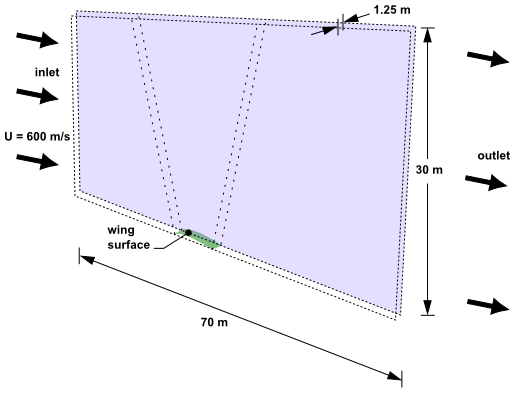
This example demonstrates the use of CFX in simulating supersonic flow over a symmetric NACA0012 airfoil at 0° angle of attack. A 2D section of the wing is modeled. A 2D hexahedral mesh is provided that you will import into CFX-Pre.
The environment is 300 K air at 1 atmosphere that passes the wing at 600 m/s. The turbulence intensity is low (.01) with an eddy length scale of .02 meters.
A mesh is provided. You will create a domain that contains three regions that will be connected by fluid-fluid interfaces. To solve the simulation, you will start with a conservative time scale that gradually increases towards the fluid residence time as the residuals decrease.
If this is the first tutorial you are working with, it is important to review the following topics before beginning:
Create a working directory.
Ansys CFX uses a working directory as the default location for loading and saving files for a particular session or project.
Download the
wing_sps.zipfile here .Unzip
wing_sps.zipto your working directory.Ensure that the following tutorial input file is in your working directory:
WingSPSMesh.out
Set the working directory and start CFX-Pre.
For details, see Setting the Working Directory and Starting Ansys CFX in Stand-alone Mode.
In CFX-Pre, select File > New Case.
Select General and click .
Select File > Save Case As.
Under File name, type
WingSPS.Click .
Right-click
Meshand select Import Mesh > Other.The Import Mesh dialog box appears.
Configure the following setting(s):
Setting
Value
Files of type
PATRAN Neutral (*out *neu)
File name
WingSPSMesh.out
Options
> Mesh Units
m
Click .
To best orient the view, right-click a blank area in the viewer and select Predefined Camera > Isometric View (Y up) from the shortcut menu.
Edit
Case Options>Generalin the Outline tree view and ensure that Automatic Default Domain is turned on. A domain namedDefault Domainshould now appear under theSimulationbranch.Edit
Default Domainand configure the following setting(s):Tab
Setting
Value
Basic Settings
Location and Type
> Location
WING_Elements
Fluid and Particle Definitions
Fluid 1
Fluid and Particle Definitions
> Fluid 1
> Material
Air Ideal Gas
Domain Models
> Pressure
> Reference Pressure [a]
1 [atm]
Fluid Models
Heat Transfer
> Option
Total Energy [b]
Turbulence
> Option
Shear Stress Transport
Click .
Create a new boundary named
Inlet.Configure the following setting(s):
Tab
Setting
Value
Basic Settings
Boundary Type
Inlet
Location
INLET
Boundary Details
Flow Regime
> Option
Supersonic
Mass And Momentum
> Option
Cart. Vel. & Pressure
Mass And Momentum
> Rel. Static Pres.
0 [Pa]
Mass And Momentum
> U
600 [m s^-1]
Mass And Momentum
> V
0 [m s^-1]
Mass And Momentum
> W
0 [m s^-1]
Turbulence
> Option
Intensity and Length Scale
Turbulence
> Fractional Intensity
0.01
Turbulence
> Eddy Length Scale
0.02 [m]
Heat Transfer
> Static Temperature
300 [K]
Click .
Create a new boundary named
Outlet.Configure the following setting(s):
Tab
Setting
Value
Basic Settings
Boundary Type
Outlet
Location
OUTLET
Boundary Details
Flow Regime
> Option
Supersonic
Click .
Create a new boundary named
SymP1.Configure the following setting(s):
Tab
Setting
Value
Basic Settings
Boundary Type
Symmetry [a]
Location
SIDE1
Click .
Create a new boundary named
SymP2.Configure the following setting(s):
Tab
Setting
Value
Basic Settings
Boundary Type
Symmetry
Location
SIDE2
Click .
Create a new boundary named
Bottom.Configure the following setting(s):
Tab
Setting
Value
Basic Settings
Boundary Type
Symmetry
Location
BOTTOM
Click .
Create a new boundary named
Top.Configure the following setting(s):
Tab
Setting
Value
Basic Settings
Boundary Type
Wall
Location
TOP
Boundary Details
Mass And Momentum
> Option
Free Slip Wall
Click .
Create a new boundary named
WingSurface.Configure the following setting(s):
Tab
Setting
Value
Basic Settings
Boundary Type
Wall
Location
WING_Nodes [a]
Click .

The imported mesh contains three regions that will be connected with domain interfaces.
Create a new domain interface named
Domain Interface 1.Configure the following setting(s):
Tab
Setting
Value
Basic Settings
Interface Type
Fluid Fluid
Interface Side 1
> Region List
Primitive 2D A
Interface Side 2
> Region List
Primitive 2D, Primitive 2D B
Click .
For high-speed compressible flow, the CFX-Solver usually requires sensible initial conditions to be set for the velocity field.
Click Global Initialization
 .
.Configure the following setting(s):
Tab
Setting
Value
Global Settings
Initial Conditions
> Cartesian Velocity Components
> Option
Automatic with Value
Initial Conditions
> Cartesian Velocity Components
> U
600 [m s^-1]
Initial Conditions
> Cartesian Velocity Components
> V
0 [m s^-1]
Initial Conditions
> Cartesian Velocity Components
> W
0 [m s^-1]
Initial Conditions
> Temperature
> Option
Automatic with Value
Initial Conditions
> Temperature
> Temperature
300 [K]
Click .
The residence time for the fluid is the length of the domain divided by the speed of the fluid; using values from the problem specification, the result is approximately:
70 [m] / 600 [m s^-1] = 0.117 [s]
In the next step, you will set a maximum timescale, then the solver will start with a conservative time scale that gradually increases towards the fluid-residence time as the residuals decrease.
Click Solver Control
 .
.Configure the following setting(s):
Tab
Setting
Value
Basic Settings
Convergence Control
> Fluid Timescale Control
> Maximum Timescale
(Selected)
Convergence Control
> Fluid Timescale Control
> Maximum Timescale
> Maximum Timescale
0.1 [s]
Convergence Criteria
> Residual Target
1.0e-05
Click .
Click Define Run
 .
.Configure the following setting(s):
Setting
Value
File name
WingSPS.def
Click .
CFX-Solver Manager automatically starts and, on the Define Run dialog box, Solver Input File is set.
If using stand-alone mode, quit CFX-Pre, saving the simulation (
.cfx) file at your discretion.
At this point, CFX-Solver Manager is running, and the Define Run dialog box is displayed, with the CFX-Solver input file set.
Click Start Run.
Select the check box next to Post-Process Results when the completion message appears at the end of the run.
If using stand-alone mode, select the check box next to Shut down CFX-Solver Manager.
Click .
The following topics will be discussed:
The first view configured shows that the bulk of the flow over the wing has a Mach Number of over 1.5.
To best orient the view, select View From -Z by typing Shift +Z.
Zoom in so the geometry fills the Viewer.
Create a new contour named
SymP2Mach.Configure the following setting(s):
Tab
Setting
Value
Geometry
Locations
SymP2
Variable
Mach Number
Range
User Specified
Min
1
Max
2
# of Contours
21
Click .
Clear the check box next to
SymP2Mach.
To display pressure information, create a contour plot that shows the pressure field:
Create a new contour named
SymP2Pressure.Configure the following setting(s):
Tab
Setting
Value
Geometry
Locations
SymP2
Variable
Pressure
Range
Global
Click .
Clear the check box next to
SymP2Pressure.
You can confirm that a significant energy loss occurs around
the wing's leading edge by plotting temperature on SymP2.
Create a new contour named
SymP2Temperature.Configure the following setting(s):
Tab
Setting
Value
Geometry
Locations
SymP2
Variable
Temperature
Range
Global
Click .
The contour shows that the temperature at the wing's leading edge is approximately 180 K higher than the inlet temperature.
Clear the check box next to
SymP2Temperature.
You can also create a user vector to show the pressure acting on the wing:
Create a new variable named
Variable 1.Configure the following setting(s):
Name Setting
Value
Variable 1
Vector
(Selected)
X Expression
(Pressure+101325[Pa])*Normal X
Y Expression
(Pressure+101325[Pa])*Normal Y
Z Expression
(Pressure+101325[Pa])*Normal Z
Click .
Create a new vector named
Vector 1.Configure the following setting(s):
Tab
Setting
Value
Geometry
Locations
WingSurface
Variable
Variable 1
Symbol
Symbol Size
0.04
Click .
Zoom in on the wing in order to see the created vector plot.