


This tutorial includes:
In this tutorial you will set up a 2D problem in which you:
Import a mesh.
Set up appropriate boundary conditions for a free surface simulation. (Free surface simulations are more sensitive to incorrect boundary and initial guess settings than other more basic models.)
Use mesh adaption to refine the mesh where the volume fraction gradient is greatest. (The refined mesh aids in the development of a sharp interface between the liquid and gas.)
Component | Feature | Details |
|---|---|---|
CFX-Pre | User Mode | General mode |
Analysis Type | Steady-state | |
Fluid Type | General Fluid | |
Domain Type | Single Domain | |
Turbulence Model | k-Epsilon | |
Heat Transfer | Isothermal | |
Buoyant Flow | ||
Multiphase | Homogeneous Model | |
Boundary Conditions | Inlet | |
Opening | ||
Outlet | ||
Symmetry Plane | ||
Wall: No Slip | ||
CEL (CFX Expression Language) | ||
Mesh Adaption | ||
Timestep | Physical Time Scale | |
CFD-Post | Plots | Default Locators |
Isosurface | ||
Polyline | ||
Sampling Plane | ||
Vector | ||
Volume | ||
Other | Chart Creation | |
Title/Text | ||
Viewing the Mesh |
This tutorial demonstrates the simulation of a free surface flow.
The geometry consists of a 2D channel in which the bottom of the channel is interrupted by a semicircular bump of radius 30 mm. The problem environment is composed of air at 1 Pa and isothermal water; the normal inlet speed is 0.26 m/s; the incoming water has a turbulence intensity of 5%. The flow upstream of the bump is subcritical. The downstream boundary conditions (the height of the water) were estimated for this tutorial; you can do this using an analytical 1D calculation or data tables for flow over a bump.
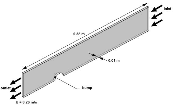
A mesh is provided. You will create a two-phase homogeneous setting and the expressions that will be used in setting initial values and boundary conditions. Later, you will use mesh adaption to improve the accuracy of the downstream simulation.
If this is the first tutorial you are working with, it is important to review the following topics before beginning:
Create a working directory.
Ansys CFX uses a working directory as the default location for loading and saving files for a particular session or project.
Download the
bump2d.zipfile here .Unzip
bump2d.zipto your working directory.Ensure that the following tutorial input files are in your working directory:
Bump2DExpressions.cclBump2Dpatran.out
Set the working directory and start CFX-Pre.
For details, see Setting the Working Directory and Starting Ansys CFX in Stand-alone Mode.
In CFX-Pre, select File > New Case.
Select General and click .
Select File > Save Case As.
Under File name, type
Bump2D.Click .
Right-click
Meshand select Import Mesh > Other.The Import Mesh dialog box appears.
Configure the following setting(s):
Setting
Value
Files of type
PATRAN Neutral (*out *neu)
Filename
Bump2Dpatran.out
Options
> Mesh units
m
Click .
To best orient the view, right-click a blank area in the viewer and select Predefined Camera > View From -Z from the shortcut menu.
Enable the display of region labels so that you can see where you will define boundaries later in this tutorial:
In the Outline tree view, edit
Case Options>Labels and Markers.Configure the following setting(s):
Tab
Setting
Value
Settings
Show Labels
(Selected)
Show Labels
> Show Primitive 3D Labels
(Selected)
Show Labels
> Show Primitive 2D Labels
(Selected)
Click .
Simulation of free surface flows usually requires defining boundary and initial conditions to set up appropriate pressure and volume fraction fields. You will need to create expressions using CEL (CFX Expression Language) to define these conditions.
In this simulation, the following conditions are set and require expressions:
An inlet boundary where the volume fraction above the free surface is 1 for air and 0 for water, and below the free surface is 0 for air and 1 for water.
A pressure-specified outlet boundary, where the pressure above the free surface is constant and the pressure below the free surface is a hydrostatic distribution. This requires you to know the approximate height of the fluid at the outlet. In this case, an analytical solution for 1D flow over a bump was used to determine the value for
DownHin Creating Expressions in CEL. The simulation is not sensitive to the exact outlet fluid height, so an approximation is sufficient. You will examine the effect of the outlet boundary condition in the postprocessing section and confirm that it does not affect the validity of the results. It is necessary to specify such a boundary condition to force the flow downstream of the bump into the supercritical regime.An initial pressure field for the domain with a similar pressure distribution to that of the outlet boundary.
Either create expressions using the Expressions workspace or read in expressions from the example file provided:
The expressions you create in this step are the same as the ones provided in Reading Expressions From a File, so you can choose to follow either set of instructions.
Right-click
Expressions, Functions and Variables>Expressionsin the tree view and select Insert > Expression.Set the name to
UpHand click to create the upstream free surface height.Set Definition to
0.069[m], and then click Apply.Use the same method to create the expressions listed in the table below. These are expressions for the downstream free surface height, the fluid density, the buoyancy reference density, the calculated density of the fluid (density - buoyancy reference density), the upstream volume fractions of air and water, the upstream pressure distribution, the downstream volume fractions of air and water, and the downstream pressure distribution.
Name
Definition
DownH
0.022 [m]
DenWater
997 [kg m^-3]
DenRef
1.185 [kg m^-3]
DenH
(DenWater - DenRef)
UpVFAir
step((y-UpH)/1[m])
UpVFWater
1-UpVFAir
UpPres
DenH*g*UpVFWater*(UpH-y)
DownVFAir
step((y-DownH)/1[m])
DownVFWater
1-DownVFAir
DownPres
DenH*g*DownVFWater*(DownH-y)
Proceed to Creating the Domain.
Set up a homogeneous, two-fluid environment:
Edit
Case Options>Generalin the Outline tree view and ensure that Automatic Default Domain is turned on. A domain namedDefault Domainshould appear under theSimulation>Flow Analysis 1branch.Double-click Default Domain.
Under Fluid and Particle Definitions, delete
Fluid 1and create a new fluid namedAir.Confirm that the following settings are configured:
Tab
Setting
Value
Basic Settings
Fluid and Particle Definitions
Air
Fluid and Particle Definitions
> Air
> Material
Air at 25 C
Click Add new item
 and create a new fluid named
 Water.Configure the following setting(s):
Tab
Setting
Value
Basic Settings
Fluid and Particle Definitions
Water
Fluid and Particle Definitions
> Water
> Material
Water [a]
Domain Models
> Pressure
> Reference Pressure
1 [atm]
Domain Models
> Buoyancy Model
> Option
Buoyant
Domain Models
> Buoyancy Model
> Gravity X Dirn.
0 [m s^-2]
Domain Models
> Buoyancy Model
> Gravity Y Dirn.[b]
-g
Domain Models
> Buoyancy Model
> Gravity Z Dirn.
0 [m s^-2]
Domain Models
> Buoyancy Model
> Buoy. Ref. Density [c]
DenRef
Fluid Models
Multiphase
> Homogeneous Model [d]
(Selected)
Multiphase
> Free Surface Model
> Option
Standard
Heat Transfer
> Option
Isothermal
Heat Transfer
> Fluid Temperature
25 [C]
Turbulence
> Option
k-Epsilon
Click .

Create a new boundary named
inflow.Configure the following setting(s):
Tab
Setting
Value
Basic Settings
Boundary Type
Inlet
Location
INFLOW
Boundary Details
Mass and Momentum
> Option
Normal Speed
Mass and Momentum
> Normal Speed
0.26 [m s^-1]
Turbulence
> Option
Intensity and Length Scale
Turbulence
> Fractional Intensity
0.05
Turbulence
> Eddy Length Scale
UpH
Fluid Values
Boundary Conditions
Air
Boundary Conditions
> Air
> Volume Fraction
> Volume Fraction
UpVFAir
Boundary Conditions
Water
Boundary Conditions
> Water
> Volume Fraction
> Volume Fraction
UpVFWater
Click .
Create a new boundary named
outflow.Configure the following setting(s):
Tab
Setting
Value
Basic Settings
Boundary Type
Outlet
Location
OUTFLOW
Boundary Details
Flow Regime
> Option
Subsonic
Mass and Momentum
> Option
Static Pressure
Mass and Momentum
> Relative Pressure
DownPres
Click .
Create a new boundary named
front.Configure the following setting(s):
Tab
Setting
Value
Basic Settings
Boundary Type
Symmetry [a]
Location
FRONT
Click .
Create a new boundary named
back.Configure the following setting(s):
Tab
Setting
Value
Basic Settings
Boundary Type
Symmetry
Location
BACK
Click .
Create a new boundary named
top.Configure the following setting(s):
Tab
Setting
Value
Basic Settings
Boundary Type
Opening
Location
TOP
Boundary Details
Mass And Momentum
> Option
Entrainment
Mass And Momentum
> Relative Pressure
0 [Pa]
Turbulence
> Option
Zero Gradient
Fluid Values
Boundary Conditions
Air
Boundary Conditions
> Air
> Volume Fraction
> Volume Fraction
1.0
Boundary Conditions
Water
Boundary Conditions
> Water
> Volume Fraction
> Volume Fraction
0.0
Click .
Create a new boundary named
bottom.Configure the following setting(s):
Tab
Setting
Value
Basic Settings
Boundary Type
Wall
Location
BOTTOM1, BOTTOM2, BOTTOM3
Boundary Details
Mass and Momentum
> Option
No Slip Wall
Wall Roughness
> Option
Smooth Wall
Click .
Set up the initial values to be consistent with the inlet boundary conditions:
Click Global Initialization
 .
.Configure the following setting(s):
Tab
Setting
Value
Global Settings
Initial Conditions
> Cartesian Velocity Components
> Option
Automatic with Value
Initial Conditions
> Cartesian Velocity Components
> U
0.26 [m s^-1] [a]
Initial Conditions
> Cartesian Velocity Components
> V
0 [m s^-1] [a]
Initial Conditions
> Cartesian Velocity Components
> W
0 [m s^-1] [a]
Initial Conditions
> Static Pressure
> Option
Automatic with Value
Initial Conditions
> Static Pressure
> Relative Pressure
UpPres
Fluid Settings
Fluid Specific Initialization
Air
Fluid Specific Initialization
> Air
> Initial Conditions
> Volume Fraction
> Option
Automatic with Value
Fluid Specific Initialization
> Air
> Initial Conditions
> Volume Fraction
> Volume Fraction
UpVFAir
Fluid Specific Initialization
Water
Fluid Specific Initialization
> Water
> Initial Conditions
> Volume Fraction
> Option
Automatic with Value
Fluid Specific Initialization
> Water
> Initial Conditions
> Volume Fraction
> Volume Fraction
UpVFWater
Click .
To improve the resolution of the interface between the air and the water, set up the mesh adaption settings:
Click Mesh Adaption
 .
.Configure the following setting(s):
Tab
Setting
Value
Basic Settings
Activate Adaption
(Selected)
Save Intermediate Files
(Cleared)
Adaption Criteria
> Variables List
Air.Volume Fraction
Adaption Criteria
> Max. Num. Steps
2
Adaption Criteria
> Option
Multiple of Initial Mesh
Adaption Criteria
> Node Factor
4
Adaption Convergence Criteria
> Max. Iter. per Step
100
Advanced Options
Node Alloc. Parameter
1.6
Number of Levels
2
Click .
Note: Setting Max. Iterations to 200 (below) and Number of (Adaption) Levels to 2 with a Max. Iter. per Step of 100 time steps each (in the previous section), results in a total maximum number of time steps of 400 (2*100+200=400).
Click Solver Control
 .
.Configure the following setting(s):
Tab
Setting
Value
Basic Settings
Convergence Control
> Max. Iterations
200
Convergence Control
> Fluid Timescale Control
> Timescale Control
Physical Timescale
Convergence Control
> Fluid Timescale Control
> Physical Timescale
0.25 [s] [a]
Advanced Options Multiphase Control
(Selected)
Multiphase Control
> Volume Fraction Coupling
(Selected)
Multiphase Control
> Volume Fraction Coupling
> Option
Coupled [b]
Estimated from the time it takes the water to flow over the bump.
The Coupled Volume Fraction solution algorithm typically converges better than the Segregated Volume Faction algorithm for buoyancy-driven problems. The Segregated Volume Faction algorithm would have required a significantly smaller timescale (0.05 [s]).
Note: Selecting these options on the solver control activates the Coupled Volume Fraction solution algorithm. This algorithm typically converges better than the Segregated Volume Faction algorithm for buoyancy-driven problems such as this tutorial. The Segregated Volume Faction algorithm would have required a 0.05 second timescale, as compared with 0.25 seconds for the Coupled Volume Fraction algorithm.
Click .
Click Define Run
 .
.Configure the following setting(s):
Setting
Value
File name
Bump2D.def
Click Save.
CFX-Solver Manager automatically starts and, on the Define Run dialog box, Solver Input File is set.
If using stand-alone mode, quit CFX-Pre, saving the simulation (
.cfx) file at your discretion.
Click Start Run.
Within 100 iterations after CFX-Solver Manager has started, the first adaption step is performed. Information written to the CFX-Solver Output file includes the number of elements refined and the size of the new mesh.
After mesh refinement, there is a jump in the residual levels. This is because the solution from the old mesh is interpolated onto the new mesh. A new residual plot also appears for the W-Mom-Bulk equation. Hexahedral mesh elements are refined orthogonally, so the mesh is no longer 2D (it is more than 1 element thick in the Z direction). Convergence to the target residual level is achieved.
It is common for convergence in a residual sense to be difficult to obtain in a free surface simulation, due to the presence of small waves at the surface preventing the residuals from dropping to the target level. This is more frequently a problem in the subcritical flow regime, as the waves can travel upstream. In the supercritical regime, the waves tend to get carried downstream and out the domain. To satisfy convergence in these cases, monitor the value of a global quantity (for example, drag for flow around a ship’s hull) to see when a steady-state value is reached.
Where there is no obvious global quantity to monitor, you should view the results to see where the solution is changing. You can do this by running transient (with time steps that are small enough to capture transient effects) for a few time steps, starting from a results file that you think is converged or from backup results files you have written at different time steps.
In both cases, look to see where the results are changing (this could be due to the presence of small transient waves). Also confirm that the value of quantities that you are interested in (for example, downstream fluid height for this case) has reached a steady-state value.
When a dialog box is displayed at the end of the run, select Post-Process Results.
If using stand-alone mode, select Shut down CFX-Solver Manager.
Click .
Display the distribution of volume fraction of water in the domain:
To best orient the view, right-click a blank area in the viewer and select Predefined Camera > View From -Z.
Zoom in so the geometry fills the viewer.
In the tree view, edit
Bump2D_001>Default Domain>front.Configure the following setting(s):
Tab
Setting
Value
Color
Mode
Variable
Variable
Water.Volume Fraction
Click .
Observe the plot, then clear the check box next to
front.
The next step involves creating a sampling plane upon which
to display velocity vectors for Water.
Select Insert > Location > Plane to create a new plane named
Plane 1.Configure the following setting(s):
Click .
Clear the check box next to
Plane 1.Create a new vector named
Vector 1.Configure the following setting(s):
Tab
Setting
Value
Geometry
Definition
> Locations
Plane 1
Definition
> Variable [a]
Water.Velocity
Symbol
Symbol Size
0.5
Because fluids in a free-surface calculation share the same velocity field, only the velocity of the first non-vapor fluid is available. The other allowed velocities are superficial velocities. For details, see Further Postprocessing.
Click .
Configure the following setting(s):
Tab
Setting
Value
Geometry
Definition
> Variable
Air.Superficial Velocity
Symbol
Symbol Size
0.15
Normalize Symbols
(Selected)
Click .
In this section, you will view the surface mesh on one of the symmetry boundaries, create volume objects to show where the mesh was modified, and create a vector plot to visualize the added mesh nodes.
Clear the check box next to
Vector 1.Zoom in so the geometry fills the Viewer.
In Outline under
Default
Domain
, editfront.Configure the following setting(s):
Tab
Setting
Value
Color
Mode
Constant
Render
Show Faces
(Cleared)
Show Mesh Lines
(Selected)
Click .
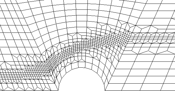
The mesh has been refined near the free surface.
In the transition region between different levels of refinement, tetrahedral and pyramidal elements are used because it is not possible to recreate hexahedral elements in CFX. Near the inlet, the aspect ratio of these elements increases.
Avoid performing mesh refinement on high-aspect-ratio hex meshes as this will produce high aspect ratio tetrahedral-elements and result in poor mesh quality.
Create a new volume named
first refinement elements.Configure the following setting(s):
Tab
Setting
Value
Geometry
Definition
> Method
Isovolume
Definition
> Variable
Refinement Level [a]
Definition
> Mode
At Value
Definition
> Value
1
Render
Show Faces
(Cleared)
Show Mesh Lines
(Selected)
Show Mesh Lines
> Line Width
2
Show Mesh Lines
> Color Mode
User Specified
Show Mesh Lines
> Line Color
(Green)
Click .
You will see a band of green, which indicates the elements that include nodes added during the first mesh adaption.
Create a new volume named
second refinement elements.Configure the following setting(s):
Tab
Setting
Value
Geometry
Definition
> Method
Isovolume
Definition
> Variable
Refinement Level
Definition
> Mode
At Value
Definition
> Value
2
Color
Color
White
Render
Show Faces
(Selected)
Show Mesh Lines
(Selected)
Show Mesh Lines
> Line Width
4
Show Mesh Lines
> Color Mode
User Specified
Show Mesh Lines
> Line Color
(Black)
Click .
You will see a band of white (with black lines); this indicates the elements that include nodes added during the second mesh adaption.
Zoom in to a region where the mesh has been refined.
The Refinement Level variable holds an integer value at each node, which is either 0, 1, or 2 (because you used a maximum of two adaption levels).
The nodal values of refinement level will be visualized next.
Create a new vector named
Vector 2.Configure the following setting(s):
Tab
Setting
Value
Geometry
Definition
> Locations
Plane 1
Definition
> Variable
(Any Vector Variable) [a]
Color
Mode
Variable
Variable
Refinement Level
Symbol
Symbol
Cube
Symbol Size
0.02
Normalize Symbols
(Selected)
Click .

In Vector 2, Blue nodes (Refinement Level
0 according to the color legend) are part of the original mesh. Green
nodes (Refinement Level 1) were added during the first adaption step.
Red nodes (Refinement Level 2) were added during the second adaption
step. Note that some elements contain combinations of blue, green,
and red nodes.
Later in this tutorial, you will create a chart to show the variation in free surface height along the channel. The data for the chart will be sampled along a polyline that follows the free surface. To make the polyline, you will use the intersection between one of the symmetry planes and an isosurface that follows the free surface. Start by creating an isosurface on the free surface:
Turn off the visibility for all objects except
Wireframe.Create a new isosurface named
Isosurface 1.Configure the following setting(s):
Tab
Setting
Value
Geometry
Definition
> Variable
Water.Volume Fraction
Definition
> Value
0.5
Click .
Creating isosurfaces using this method is a good way to visualize a free surface in a 3D simulation.
Right-click any blank area in the viewer, select Predefined Camera, then select Isometric View (Y up).
Create a polyline along the isosurface that you created in the previous step:
Turn off the visibility of
Isosurface 1.Create a new polyline named
Polyline 1.Configure the following setting(s):
Tab
Setting
Value
Geometry
Method
Boundary Intersection
Boundary List
front
Intersect With
Isosurface 1
Click .
A green line is displayed that follows the high-Z edge of the isosurface.
Create a chart that plots the free surface height using the polyline that you created in the previous step:
Create a new chart named
Chart 1.The Chart Viewer is displayed.
Configure the following setting(s):
Tab
Setting
Value
General
Title
Free Surface Height for Flow over a Bump
Data Series
Name
free surface height
Location
Polyline 1
X Axis
Variable
X
Y Axis
Variable
Y
Line Display
Symbols
Rectangle
Click .
As discussed in Creating Expressions for Initial and Boundary Conditions, an approximate outlet elevation is imposed as part of the boundary, even though the flow is supercritical. The chart illustrates the effect of this, in that the water level rises just before the exit plane. It is evident from this plot that imposing the elevation does not affect the upstream flow.
The chart shows a wiggle in the elevation of the free surface interface at the inlet. This is related to an over-specification of conditions at the inlet because both the inlet velocity and elevation were specified. For a subcritical inlet, only the velocity or the total energy should be specified. The wiggle is due to a small inconsistency between the specified elevation and the elevation computed by the solver to obtain critical conditions at the bump. The wiggle is analogous to one found if pressure and velocity were both specified at a subsonic inlet in a converging-diverging nozzle with choked flow at the throat.
You may want to create some plots using the <Fluid>.Superficial
Velocity variables. This is the fluid volume fraction multiplied
by the fluid velocity and is sometimes called the volume flux. It
is useful to use this variable for vector plots in separated multiphase
flow, as you will only see a vector where a significant amount of
that phase exists.
Tip: You can right-click an existing vector plot and select a new vector variable.
For supercritical free surface flows, the supercritical outlet boundary is usually the most appropriate boundary for the outlet because it does not rely on the specification of the outlet pressure distribution (which depends on an estimate of the free surface height at the outlet). The supercritical outlet boundary requires a relative pressure specification for the gas only; no pressure information is required for the liquid at the outlet. For this tutorial, the relative gas pressure at the outlet should be set to 0 Pa.
The supercritical outlet condition may admit multiple solutions. To find the supercritical solution, it is often necessary to start with a static pressure outlet condition (as previously done in this tutorial) or an average static pressure condition where the pressure is set consistent with an elevation to drive the solution into the supercritical regime. The outlet condition can then be changed to the supercritical option.