


This tutorial includes:
In this tutorial you will learn about:
Using a rough wall boundary in CFX-Pre to simulate the pipe wall
Creating a fully developed inlet velocity profile using the CFX Expression Language
Setting up a Particle Tracking simulation in CFX-Pre to trace sand particles
Animating particle tracks in CFD-Post to trace sand particles through the domain
Performing quantitative calculation of average static pressure in CFD-Post on the outlet boundary.
|
Component |
Feature |
Details |
|---|---|---|
|
CFX-Pre |
User Mode |
General mode |
|
Analysis Type |
Steady State | |
|
Fluid Type |
General Fluid | |
|
Domain Type |
Single Domain | |
|
Turbulence Model |
k-Epsilon | |
|
Heat Transfer |
None | |
|
Particle Tracking | ||
|
Boundary Conditions |
Inlet (Profile) | |
|
Inlet (Subsonic) | ||
|
Outlet (Subsonic) | ||
|
Symmetry Plane | ||
|
Wall: No-Slip | ||
|
Wall: Rough | ||
|
CEL (CFX Expression Language) | ||
|
Timestep |
Auto Time Scale | |
|
CFD-Post |
Plots |
Animation |
|
Default Locators | ||
|
Particle Track | ||
|
Point | ||
|
Slice Plane | ||
|
Other |
Changing the Color Range | |
|
Movie Generation | ||
|
Particle Track Animation | ||
|
Quantitative Calculation | ||
|
Symmetry, Reflection Plane |
Pumps and compressors are commonplace. An estimate of the pumping requirement can be calculated based on the height difference between source and destination and head loss estimates for the pipe and any obstructions/joints along the way. Investigating the detailed flow pattern around a valve or joint however, can lead to a better understanding of why these losses occur. Improvements in valve/joint design can be simulated using CFD, and implemented to reduce pumping requirements and cost.
Flows can contain particulates that affect the flow and cause erosion to pipe and valve components. You can use the particle-tracking capability of CFX to simulate these effects.
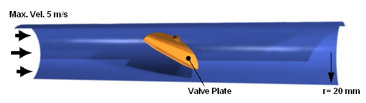
In this example, water flows at 5 m/s through a 20 mm radius pipe that has a rough internal surface. The velocity profile is assumed to be fully developed at the pipe inlet. The flow, which is controlled by a butterfly valve set at an angle of 55° to the vertical axis, contains sand particles ranging in size from 50 to 500 microns. The equivalent sand grain roughness is 0.2 mm.
The reference temperature is 300 K; the reference pressure is 1 atm.
A mesh is provided. You will create sand particles and a domain that contains water; for one part of the simulation the water and sand will be fully coupled, and for the other part of the simulation they will be one-way coupled. To increase the accuracy of the simulation, the inlet will be given a velocity profile that simulates a fully-developed boundary layer.
To solve the simulation, you will create two sets of identical particles. The first set will be fully coupled to predict the effect of the particles on the continuous phase flow field and enable the particles to influence the flow field. The second set will be one-way coupled but will contain a much higher number of particles to provide a more accurate calculation of the particle volume fraction and local forces on walls, but without affecting the flow field.
If this is the first tutorial you are working with, it is important to review the following topics before beginning:
Create a working directory.
Ansys CFX uses a working directory as the default location for loading and saving files for a particular session or project.
Download the
pipe_valve.zipfile here .Unzip
pipe_valve.zipto your working directory.Ensure that the following tutorial input file is in your working directory:
PipeValveMesh.gtm
Set the working directory and start CFX-Pre.
For details, see Setting the Working Directory and Starting Ansys CFX in Stand-alone Mode.
In CFX-Pre, select File > New Case.
Select General and click .
Select File > Save Case As.
Under File name, type
PipeValve.Click .
Right-click
Meshand select Import Mesh > CFX Mesh.The Import Mesh dialog box appears.
Configure the following setting(s):
Setting
Value
File name
PipeValveMesh.gtm
Click .
The material properties of the sand particles used in the simulation need to be defined. Heat transfer and radiation modeling are not used in this simulation, so the only properties that need to be defined are the density of the sand and the diameter range.
To calculate the effect of the particles on the continuous fluid, between 100 and 1000 particles are usually required. However, if accurate information about the particle volume fraction or local forces on wall boundaries is required, then a much larger number of particles must be modeled.
When you create the domain, choose either full coupling or one-way coupling between the particle and continuous phase. Full coupling is needed to predict the effect of the particles on the continuous phase flow field but has a higher CPU cost than one-way coupling; one-way coupling simply predicts the particle paths during postprocessing based on the flow field, but without affecting the flow field.
To optimize CPU usage, you can create two sets of identical particles. The first set should be fully coupled and around 200 particles will be used. This allows the particles to influence the flow field. The second set uses one-way coupling but contains 5000 particles. This provides a more accurate calculation of the particle volume fraction and local forces on walls. (These values are defined in the inlet boundary definition.)
For this tutorial you will create a "Sand Fully Coupled" boundary condition that has 200 particles moving with a mass flow rate of 0.01 kg/s and a "Sand One Way Coupled" boundary condition that has 5000 particles moving with a mass flow rate of 0.01 kg/s. In both cases the sand density is 2300 [kg m^-3]; particle diameters range from 50 e-6 m to 500 e-6 m, with an average diameter of 250 e-6 m and a standard deviation of 70 e-6 m. You will set a Finnie erosion model with a velocity power factor of 2 and a reference velocity of 1 m/s.
Click Insert Material
 then create a new material named
 Sand Fully Coupled.Configure the following setting(s):
Tab
Setting
Value
Basic Settings
Material Group
Particle Solids
Thermodynamic State
(Selected)
Material Properties
Thermodynamic Properties
> Equation of State
> Density
2300 [kg m^-3] [ a ]
Thermodynamic Properties
> Specific Heat Capacity
(Selected)
Thermodynamic Properties
> Specific Heat Capacity
> Specific Heat Capacity
0 [J kg^-1 K^-1] [ b ]
Thermodynamic Properties
> Reference State
(Selected)
Thermodynamic Properties
> Reference State
> Option
Specified Point
Thermodynamic Properties
> Reference State
> Ref. Temperature
300 [K] [ a ]
Click .
Under
Materials, right-clickSand Fully Coupledand select Duplicate from the shortcut menu.Rename the duplicate as
Sand One Way Coupled.Sand One Way Coupledis created with properties identical toSand Fully Coupled.
Set up an environment that has water and sand defined in two ways; one in which the sand is fully coupled, and one in which the sand is one-way coupled:
Edit
Case Options>Generalin the Outline tree view and ensure that Automatic Default Domain is turned on. A domain namedDefault Domainshould appear under theSimulation>Flow Analysis 1branch.Double-click
Default Domain.Under Fluid and Particle Definitions, delete
Fluid 1.Click Add new item
 to create a new fluid definition
named
to create a new fluid definition
named Water.Set Fluid and Particle Definitions > Water > Material to
Water.Create a new fluid definition named
Sand Fully Coupled.Under Fluid and Particle Definitions > Sand Fully Coupled, configure the following setting(s):
Setting
Value
Material
Sand Fully Coupled [ a ]
Morphology
> Option
Particle Transport Solid
Morphology
> Particle Diameter Distribution
(Selected)
Morphology
> Particle Diameter Distribution
> Option
Normal in Diameter by Mass
Morphology
> Particle Diameter Distribution
> Minimum Diameter
50e-6 [m]
Morphology
> Particle Diameter Distribution
> Maximum Diameter
500e-6 [m]
Morphology
> Particle Diameter Distribution
> Mean Diameter
250e-6 [m]
Morphology
> Particle Diameter Distribution
> Std. Deviation
70e-6 [m]
Create a new fluid definition named
Sand One Way Coupled.Under Fluid and Particle Definitions > Sand One Way Coupled, configure the following setting(s):
Setting
Value
Material
Sand One Way Coupled [ a ]
Morphology
> Option
Particle Transport Solid
Morphology
> Particle Diameter Distribution
(Selected)
Morphology
> Particle Diameter Distribution
> Option
Normal in Diameter by Mass
Morphology
> Particle Diameter Distribution
> Minimum Diameter
50e-6 [m]
Morphology
> Particle Diameter Distribution
> Maximum Diameter
500e-6 [m]
Morphology
> Particle Diameter Distribution
> Mean Diameter
250e-6 [m]
Morphology
> Particle Diameter Distribution
> Std. Deviation
70e-6 [m]
Configure the following setting(s):
Tab
Setting
Value
Basic Settings
Domain Models
> Pressure
> Reference Pressure
1 [atm]
Fluid Models
Heat Transfer
> Option
None
Turbulence
> Option
k-Epsilon[ a ]
Fluid Specific Models
Fluid
Sand Fully Coupled
Fluid
> Sand Fully Coupled
> Erosion Model
> Option
Finnie
Fluid
> Sand Fully Coupled
> Erosion Model
> Vel. Power Factor
2.0
Fluid
> Sand Fully Coupled
> Erosion Model
> Reference Velocity
1 [m s^-1]
Fluid
> Sand One Way Coupled
(Selected)
Fluid
> Sand One Way Coupled
> Erosion Model
> Option
Finnie
Fluid
> Sand One Way Coupled
> Erosion Model
> Vel. Power Factor
2.0
Fluid
> Sand One Way Coupled
> Erosion Model
> Reference Velocity
1 [m s^-1]
Fluid Pair Models
Fluid Pair
Water | Sand Fully Coupled
Fluid Pairs
> Water | Sand Fully Coupled
> Particle Coupling
Fully Coupled
Fluid Pairs
>Water | Sand Fully Coupled
> Momentum Transfer
> Drag Force
> Option
Schiller Naumann [ b ]
Fluid Pair
Water | Sand One Way Coupled
Fluid Pairs
> Water | Sand One Way Coupled
> Particle Coupling
One-way Coupling
Fluid Pairs
> Water | Sand One Way Coupled
> Momentum Transfer
> Drag Force
> Option
Schiller Naumann [ b ]
Click .
In previous tutorials you have often defined a uniform velocity profile at an inlet boundary. This means that the inlet velocity near to the walls is the same as that at the center of the inlet. If you look at the results from these simulations, you will see that downstream of the inlet a boundary layer will develop, so that the downstream near wall velocity is much lower than the inlet near wall velocity.
You can simulate an inlet more accurately by defining an inlet velocity profile, so that the boundary layer is already fully developed at the inlet. The one seventh power law will be used in this tutorial to describe the profile at the pipe inlet. The equation for this is:
 | (11–1) |
where  is the pipe
centerline velocity,
is the pipe
centerline velocity,  is the pipe
radius, and
is the pipe
radius, and  is the distance from the pipe
centerline.
is the distance from the pipe
centerline.
You can create a non-uniform (profile) boundary condition by doing one of the following:
Creating an expression using CEL that describes the inlet profile. Using a CEL expression is the easiest way to create the profile.
Creating a User CEL Function that uses a user subroutine (linked to the CFX-Solver during execution) to describe the inlet profile. The User CEL Function method is more complex, but is provided here as an example of how to use this feature.
Loading a boundary condition profile file (a file that contains boundary condition profile data).
Profiles created from data files are not used in this tutorial, but are used in the tutorial Flow in a Process Injection Mixing Pipe.
Note: For complex profiles, it may be necessary to use a User CEL Function or a boundary condition profile file.
Use a CEL expression to define the velocity profile for the inlet boundary:
Click Insert Expression
 and create the following expressions using Equation 11–1 and values from the problem description:
Name
Definition
Rmax
20 [mm]
Wmax
5 [m s^-1]
Wprof
Wmax*(abs(1-r/Rmax)^0.143)
In the definition of
Wprof, the variable r (radius) is a CFX System Variable defined as:
(11–2)
In this equation,
 and
and  are defined as directions
1 and 2 (X and Y for Cartesian coordinate frames) respectively, in
the selected reference coordinate frame.
are defined as directions
1 and 2 (X and Y for Cartesian coordinate frames) respectively, in
the selected reference coordinate frame.Continue with the tutorial at Creating the Boundary Conditions.
Create a new boundary named
inlet.Configure the following setting(s):
Tab
Setting
Value
Basic Settings
Boundary Type
Inlet
Location
inlet
Boundary Details
Mass And Momentum
> Option
Cart. Vel. Components
Mass And Momentum
> U
0 [m s^-1]
Mass And Momentum
> V
0 [m s^-1]
Mass And Momentum
> W
Wprof [ a ]
Fluid Values [ b ]
Boundary Conditions
Sand Fully Coupled
Boundary Conditions
> Sand Fully Coupled
> Particle Behavior
> Define Particle Behavior
(Selected)
Boundary Conditions
> Sand Fully Coupled
> Mass and Momentum
> Option
Cart. Vel. Components [ c ]
Boundary Conditions
> Sand Fully Coupled
> Mass And Momentum
> U
0 [m s^-1]
Boundary Conditions
> Sand Fully Coupled
> Mass And Momentum
> V
0 [m s^-1]
Boundary Conditions
> Sand Fully Coupled
> Mass And Momentum
> W
Wprof [ a ]
Boundary Conditions
> Sand Fully Coupled
> Particle Position
> Option
Uniform Injection
Boundary Conditions
> Sand Fully Coupled
> Particle Position
> Number of Positions
> Option
Direct Specification
Boundary Conditions
> Sand Fully Coupled
> Particle Position
> Number of Positions
> Number
200
Boundary Conditions
> Sand Fully Coupled
> Particle Mass Flow
> Mass Flow Rate
0.01 [kg s^-1]
Boundary Conditions
Sand One Way
Coupled
Boundary Conditions
> Sand One Way Coupled
> Particle Behavior
> Define Particle Behavior
(Selected)
Boundary Conditions
> Sand One Way Coupled
> Mass and Momentum
> Option
Cart. Vel. Components [ c ]
Boundary Conditions
> Sand One Way Coupled
> Mass And Momentum
> U
0 [m s^-1]
Boundary Conditions
> Sand One Way Coupled
> Mass And Momentum
> V
0 [m s^-1]
Boundary Conditions
> Sand One Way Coupled
> Mass And Momentum
> W
Wprof [ a ]
Boundary Conditions
> Sand One Way Coupled
> Particle Position
> Option
Uniform Injection
Boundary Conditions
> Sand One Way Coupled
> Particle Position
> Number of Positions
> Option
Direct Specification
Boundary Conditions
> Sand One Way Coupled
> Particle Position
> Number of Positions
> Number
5000
Boundary Conditions
> Sand One Way Coupled
> Particle Position
> Particle Mass Flow Rate
> Mass Flow Rate
0.01 [kg s^-1]
Click .
One-way coupled particles are tracked as a function of the fluid flow field. The latter is not influenced by the one-way coupled particles. The fluid flow will therefore be influenced by the 0.01 [kg s^-1] flow of two-way coupled particles, but not by the 0.01 [kg s^-1] flow of one-way coupled particles.
Create a new boundary named
outlet.Configure the following setting(s):
Tab
Setting
Value
Basic Settings
Boundary Type
Outlet
Location
outlet
Boundary Details
Flow Regime
> Option
Subsonic
Mass and Momentum
> Option
Average Static Pressure
Mass and Momentum
> Relative Pressure
0 [Pa]
Click .
Create a new boundary named
symP.Configure the following setting(s):
Tab
Setting
Value
Basic Settings
Boundary Type
Symmetry [ a ]
Location
symP
Click .
Create a new boundary named
pipe wall.Configure the following setting(s):
Tab
Setting
Value
Basic Settings
Boundary Type
Wall
Location
pipe wall
Boundary Details
Wall Roughness
> Option
Rough Wall
Wall Roughness
> Sand Grain Roughness
0.2 [mm] [ a ]
Fluid Values
Boundary Conditions
Sand Fully Coupled
Boundary Conditions
> Sand Fully Coupled
> Velocity
> Option
Restitution Coefficient
Boundary Conditions
> Sand Fully Coupled
> Velocity
> Perpendicular Coeff.
0.8 [ b ]
Boundary Conditions
> Sand Fully Coupled
> Velocity
> Parallel Coeff.
1
Apply the same setting values for
Sand One Way Coupledas forSand Fully Coupled.Click .
In the Outline tree view, edit the boundary named
Default Domain Default.Configure the following setting(s):
Tab
Setting
Value
Fluid Values
Boundary Conditions
Sand Fully Coupled
Boundary Conditions
> Sand Fully Coupled
> Velocity
> Perpendicular Coeff.
0.9 [ a ]
Boundary Conditions
Sand One Way Coupled
Boundary Conditions
> Sand One Way Coupled
> Velocity
> Perpendicular Coeff.
0.9
Click .
Set up the initial values to be consistent with the inlet boundary conditions:
Click Global Initialization
 .
.Configure the following setting(s):
Tab
Setting
Value
Global Settings
Initial Conditions
> Cartesian Velocity Components
> Option
Automatic with Value
Initial Conditions
> Cartesian Velocity Components
> Option
> U
0 [m s^-1]
Initial Conditions
> Cartesian Velocity Components
> Option
> V
0 [m s^-1]
Initial Conditions
> Cartesian Velocity Components
> Option
> W
Wprof
Click .
Click Solver Control
 .
.Configure the following setting(s):
Tab
Setting
Value
Basic Settings
Advection Scheme
> Option
High Resolution
Particle Control
Particle Integration
> Max. Particle Intg. Time Step
(Selected)
Particle Integration
> Max. Particle Intg. Time Step
> Value
1e+10 [s]
Particle Termination Control
(Selected)
Particle Termination Control
> Maximum Tracking Time
(Selected)
Particle Termination Control
> Maximum Tracking Time
> Value
10 [s]
Particle Termination Control
> Maximum Tracking Distance
(Selected)
Particle Termination Control
> Maximum Tracking Distance
> Value
10 [m]
Particle Termination Control
> Max. Num. Integration Steps
(Selected)
Particle Termination Control
> Max. Num. Integration Steps
> Value
10000 [ a ]
Note: The numeric values in the preceding table are all designed to put a high upper limit on the amount of processing that will be done. For example, the tracking time of 10 seconds would enable a particle to get caught in an eddy for a reasonable amount of time.
Click .
Click Define Run
 .
.Configure the following setting(s):
Setting
Value
File name
PipeValve.def
Click .
CFX-Solver Manager automatically starts and, on the Define Run dialog box, Solver Input File is set.
If using stand-alone mode, quit CFX-Pre, saving the simulation (
.cfx) file at your discretion.
When CFX-Pre has shut down and CFX-Solver Manager has started, you can obtain a solution to the CFD problem by using the procedure that follows.
Ensure the Define Run dialog box is displayed and click Start Run.
Select the check box next to Post-Process Results when the completion message appears at the end of the run.
If using stand-alone mode, select the check box next to Shut down CFX-Solver Manager.
Click .
In this section, you will first plot erosion on the valve surface and side walls due to the sand particles. You will then create an animation of particle tracks through the domain.
An important consideration in this simulation is erosion to
the pipe wall and valve due to the sand particles. A good indication
of erosion is given by the Erosion Rate Density parameter, which corresponds to pressure and shear stress due to
the flow.
Edit the object named
Default Domain Default.Configure the following setting(s) using the Ellipsis
 as required for variable selection:
Click .
As can be seen, the highest values occur on the edges of the valve where most particles strike. Erosion of the low Z side of the valve would occur more quickly than for the high Z side.
Set the user specified range for coloring to resolve areas of stress on the pipe wall near of the valve:
Ensure that the check box next to
Res PT for
Sand Fully Coupled
is cleared.Clear the check box next to
Default Domain Default.Edit the object named
pipe wall.Configure the following setting(s):
Tab
Setting
Value
Color
Mode
Variable
Variable
Sand One Way Coupled.Erosion Rate Density
Range
User Specified
Min
0 [kg m^-2 s^-1]
Max
25 [kg m^-2 s^-1]
Click .
Optionally, fill the check box next to
Default Domain Defaultto see how sand particles have deflected off the butterfly valve then to the pipe wall.
Default particle track objects are created at the start of the
session. One particle track is created for each set of particles in
the simulation. You are going to make use of the default object for Sand Fully Coupled.
The default object draws 25 tracks as lines from the inlet to outlet. The Info tab shows information about the total number of tracks, the index range, and the track numbers that are drawn.
Turn off the visibility for all objects except
Wireframe.Edit the object named
Res PT for Sand Fully Coupled.Configure the following setting(s):
Tab
Setting
Value
Geometry
Max Tracks
20 [ a ]
Color
Mode
Variable
Variable
Sand Fully Coupled.Velocity w
Symbol
Show Symbols
(Selected)
Show Symbols
> Max Time
0 [s]
Show Symbols
> Min Time
0 [s]
Show Symbols
> Interval
0.07 [s]
Show Symbols
> Symbol
Ball
Show Symbols
> Scale
1.2
Click .
Right-click a blank area anywhere in the viewer, select Predefined Camera from the shortcut menu and select View From +X to view the particle tracks.
Symbols can be seen at the start of each track.
The following steps describe how to create a particle tracking animation using Sweep Animation. Similar effects can be achieved in more detail using the Keyframe Animation option, which allows full control over all aspects on an animation.
Right-click a blank area in the viewer and select Predefined Camera > Isometric View (Y up) from the shortcut menu.
Right-click an edge of the flat side on the half cylinder and select Reflect/Mirror from the shortcut menu. Click X Axis to choose it as the normal direction.
Note: Alternatively, you can apply Reflect/Mirror, by double-clicking
Default Domainto open the details view. In the Instancing tab enable Apply Reflection and select Method toYZ Plane. Click Apply.Select Tools > Animation or click Animation
 .
.The Animation dialog box appears.
Set Type to Sweep Animation.
Select
Res PT for Sand Fully Coupled:Click Options to display the Animation Options dialog box, then clear Override Symbol Settings to ensure the symbol type and size are kept at their specified settings for the animation playback. Click .
Note: The arrow pointing downward in the bottom right corner of the Animation Window will reveal the Options button if it is not immediately visible.
Select Loop.
Clear Repeat forever
 and ensure that Repeat is set
to
and ensure that Repeat is set
to 1.Select Save Movie.
Set Format to
MPEG1.Click Browse
 and
enter
and
enter tracks.mpgas the filename.Click Play the animation
 .
.If prompted to overwrite an existing movie, click Overwrite.
The animation plays and builds an
.mpgfile.Close the Animation dialog box.
On the outlet boundary you created in CFX-Pre, you set the Average Static Pressure to 0.0 [Pa]. To see the effect of this:
From the main menu select Tools > Function Calculator.
The Function Calculator is displayed. It enables you to perform a wide range of quantitative calculations on your results.
Note: You should use Conservative variable values when performing calculations and Hybrid values for visualization purposes. Conservative values are set by default in CFD-Post but you can manually change the setting for each variable in the Variables Workspace, or the settings for all variables by using the Function Calculator.
Set Function to
maxVal.Set Location to
outlet.Set Variable to
Pressure.Click Calculate.
The result is the maximum value of pressure at the outlet.
Perform the calculation again using
minValto obtain the minimum pressure at the outlet.Select
areaAve, and then click Calculate.This calculates the area weighted average of pressure.
The average pressure is approximately zero, as specified by the boundary.
The geometry was created using a symmetry plane. In addition
to the Reflect/Mirror option from
the shortcut menu, you also can display the other half of the geometry
by creating a YZ Plane at X = 0 and then editing
the Default Transform object to use this plane
as a reflection plane.
When you have finished viewing the results, quit CFD-Post.