


This tutorial includes:
Important: This tutorial requires file TimeInletDistIni_001.res, which is produced by following tutorial Time Transformation Method for an Inlet Disturbance Case.
In this tutorial you will learn about:
Component | Feature | Details |
|---|---|---|
CFX-Pre | User Mode | Turbo Wizard |
General Mode | ||
Analysis Type | Transient Blade Row | |
Fluid Type | Air Ideal Gas | |
Domain Type | Single Domain | |
Stationary Frame | ||
Turbulence Model | k-Epsilon | |
Heat Transfer | Total Energy | |
Boundary Conditions | Inlet (Subsonic) | |
Outlet (Subsonic) | ||
CFD-Post | Plots | Contour |
Animation |
The goal of this tutorial is to set up a transient blade row calculation to model an inlet disturbance (frozen gust) using the Fourier Transformation model. The tutorial uses an axial turbine to illustrate the basic concepts of setting up, running, and monitoring a transient blade row problem in Ansys CFX. The full geometry of the axial rotor-stator stage contains 21 stator blades and 28 rotor blades.
In this tutorial, rotational phase-shifted periodic boundaries are used to enable only a small section of the full geometry to be modeled. The schematic below shows three stator blades along with the profile boundary showing a disturbance in the total temperature of the flow:
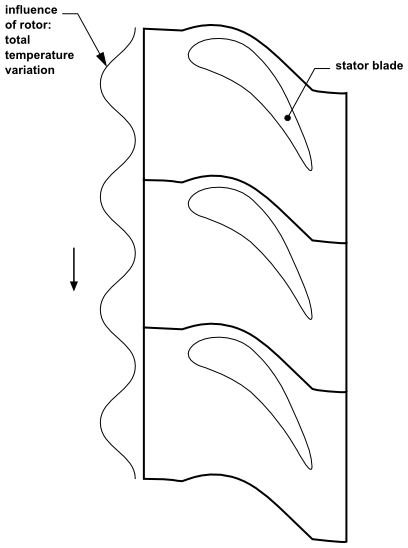
The geometry to be modeled consists of the stator blade row. When using the Fourier Transformation model, two passages of the bladed geometry must be used. This is required to enable a clean signal to accumulate at the sampling interface between the two passages where the Fourier coefficients will also be accumulated. In the stator blade component, a 34.28° section is being modeled (2*360°/21 blades). The rotor is upstream of the stator and creates a disturbance in the total temperature of the flow, which is then imposed at the inlet.
The flow is modeled as being turbulent and compressible. The inlet boundary condition serves to model the disturbance coming from the upstream rotor. It consists of a total temperature Gaussian profile with a pitch of 12.86° (360°/28 blades) and rotating about the Z axis at 6300 [rev min^-1]. The outlet boundary condition is a static pressure profile. The inlet and outlet boundary profiles are provided in .csv files. The outlet boundary profile was obtained from a previous simulation of a downstream stage.
When starting a new run, it is good practice to initialize Transient Blade Row simulations using results from steady-state cases. In this case, you will incorporate the steady-state results obtained from a previous tutorial. You will also use the Turbomachinery wizard feature, which facilitates the setup of a Fourier Transformation simulation. In order to do this, you have to:
Define the Transient Blade Row simulation using the Turbomachinery wizard in CFX-Pre.
Import the stator mesh, which was created in Ansys TurboGrid.
Enter the basic model definition.
Set the profile boundary conditions using CFX-Pre in General mode.
Run the transient blade row simulation using the steady-state results from Time Transformation Method for an Inlet Disturbance Case as an initial guess.
Create a working directory.
Ansys CFX uses a working directory as the default location for loading and saving files for a particular session or project.
Download the
fourier_inlet_disturbance.zipfile here .Unzip
fourier_inlet_disturbance.zipto your working directory.Ensure that the following tutorial input files are in your working directory:
TBRInletDistInlet.csvTBRInletDistOutlet.csvTBRInletDistStator.gtmTimeInletDistIni_001.res(produced by following tutorial Time Transformation Method for an Inlet Disturbance Case)
Set the working directory and start CFX-Pre.
For details, see Setting the Working Directory and Starting Ansys CFX in Stand-alone Mode.
The following sections describe the transient blade row simulation setup in CFX-Pre.
This tutorial uses the Turbomachinery wizard in CFX-Pre. This preprocessing mode is designed to simplify the setup of turbomachinery simulations.
In CFX-Pre, select File > New Case.
Select TurboMachinery and click OK.
Select File > Save Case As.
Under File name, type
FourierInletDist.Click Save.
In the Basic Settings panel, configure the following:
Setting
Value
Machine Type
Axial Turbine
Axes
> Rotation Axis
Z
Analysis Type
> Type
Transient Blade Row
Analysis Type
> Method
Fourier Transformation
Click .
The Fourier Transformation method requires two stator blade passages. You will define a new component and import the stator mesh.
Right-click in the blank area and select Add Component from the shortcut menu.
Create a new component of type
Stationary, namedS1and click .Configure the following setting(s):
Setting
Value
Mesh
> File
TBRInletDistStator.gtm[a]
Expand the Passages and Alignment section.
Click Edit.
Configure the following setting(s):
Setting
Value
Passages and Alignment
> Passages to Model
2
Click Done
You will see that the stator blade passage is correctly replicated and the resulting mesh now contains two stator blade passages. This will also create the Sampling Interface (S1 Internal Interface 1) required for the Fourier Transformation model.
Click .
In this section, you will set properties of the fluid domain and some solver parameters.
In the Physics Definition panel, configure the following setting(s):
Setting
Value
Fluid
Air Ideal Gas
Model Data
> Reference Pressure
0 [atm][a]
Model Data
> Heat Transfer
Total Energy
Model Data
> Turbulence
k-Epsilon
Inflow/Outflow Boundary Templates
> P-Total Inlet P-Static Outlet
(Selected)
Inflow/Outflow Boundary Templates
> Inflow
> P-Total
200000 [Pa]
Inflow/Outflow Boundary Templates
> Inflow
> T-Total
500 [K] [b]
Inflow/Outflow Boundary Templates
> Inflow
> Flow Direction
Cylindrical Components
Inflow/Outflow Boundary Templates
> Inflow Direction (a,r,t)
1, 0, -0.4
Inflow/Outflow Boundary Templates
> Outflow
> P-Static
175000 [Pa] [b]
Click .
Under the Interface Definition section you can observe that both the Fourier coefficient sampling interface S1 Internal Interface 1 as well as the phase shifted interface S1 to S1 Periodic 1 are automatically created.
Click Next.
In this section, you will specify the periodicity of the disturbance being imposed. In this case the inlet profile has a pitch of 12.857 [Degrees] or 1/28 of the wheel, so you need to specify 28 for the value of Passages in 360.
Configure the following setting(s):
Setting
Value
Disturbances
> External Boundary
> Passages in 360
28
Continue clicking until the Final Operations panel is reached.
Ensure that Operation is set to
Enter General Modebecause you will continue to define the simulation through settings not available in the TurboMachinery wizard.Click Finish.
Note: You may ignore the physics validation errors for the moment. You will correct these errors in the steps that follow.
You will include additional settings to improve the accuracy of the simulation.
Edit
S1.Configure the following setting(s):
Tab
Setting
Value
Fluid Models
Heat Transfer
> Incl. Viscous Work Term
(Selected)
Turbulence
> High Speed (compressible) Wall Heat Transfer Model
(Selected)
Click .
The inlet and outlet boundary conditions are defined using profiles in your working directory. Boundary profile data must be initialized before they can be used for boundary conditions.
Select > .
The Initialize Profile Data dialog box appears.
Beside Profile Data File, click Browse
 .
.The Select Profile Data File dialog box appears.
From your working directory, select TBRInletDistOutlet.csv.
Click .
Click .
The outlet profile data is read into memory.
Next, you will prepare the inlet profile. Since the supplied profile file, TBRInletDistInlet.csv, only covers a single passage, you need to expand the profile so that it covers at least both passages. In this case you will expand the profile so that it covers the full wheel.
Select > .
The Edit Profile Data dialog box appears.
Under Source Profile, click Browse
.The Select Profile Data File dialog box appears.
From your working directory, select TBRInletDistInlet.csv and click Open.
Set Write to Profile to
TBRInletDistInlet_FullWheel.csv.Ensure that Initialize New Profile After Writing is selected so that the inlet profile data will be automatically initialized using the expanded profile.
In the Transformations frame, click Add new item
 , set Name to
 Transformation 1, and click OK.Configure the following setting(s):
Setting
Value
Transformation 1
> Option
Expansion
Transformation 1
> Expansion Definition
> Rotation Option
Principal Axis
Transformation 1
> Expansion Definition
> Axis
Z
Transformation 1
> Expansion Definition
> Passages in Profile
1
Transformation 1
> Expansion Definition
> Passages in 360
28
Transformation 1
> Expansion Definition
> Expansion Option
Expand to Full Circle
Transformation 1
> Expansion Definition
> Theta Offset
0 [degree]
Click .
Note: After profile data has been initialized from a file, the profile data file should not be deleted or otherwise removed from its directory. By default, the full file path to the profile data file is stored in CFX-Pre, and the profile data file is read directly by CFX-Solver each time the solver is started or restarted.
Create a local rotating coordinate frame that will be applied to the inlet boundary in order to cause it to rotate:
Select Insert > Coordinate Frame.
Accept the default name and click .
Configure the following setting(s):
Setting
Value
Option
Axis Points
Coord Frame Type
Cartesian
Ref. Coordinate Frame
Coord 0
Origin
0, 0, 0
Z Axis Point
0, 0, 1
X-Z Plane Pt
1, 0, 0
Frame Motion
(Selected)
Frame Motion
> Option
Rotating
Frame Motion
> Angular Velocity
6300 [rev min^-1]
Frame Motion
> Axis Definition
> Option
Coordinate Axis
Frame Motion
> Axis Definition
> Rotation Axis
Global Z
Click .
Here, you will apply profiles to the inlet and outlet boundary conditions. In addition to this, you will also be applying the local rotating frame to the inlet boundary.
Edit
S1 Inlet.Configure the following setting(s):
Tab
Setting
Value
Basic Settings
Profile Boundary Conditions
> Use Profile Data
(Selected)
Profile Boundary Setup
> Profile Name
inletTo
Click .
You can create a moving disturbance by applying a moving coordinate frame to a boundary. Add rotational motion to the boundary condition values on the inlet by applying the local rotating coordinate frame that you made earlier:
Configure the following setting(s):
Tab
Setting
Value
Basic Settings
Coordinate Frame
(Selected)
Coordinate Frame
> Coordinate Frame
Coord 1
Click .
Edit
S1 Outlet.Configure the following setting(s):
Tab
Setting
Value
Basic Settings
Profile Boundary Conditions
> Use Profile Data
(Selected)
Profile Boundary Setup
> Profile Name
outlet
Click .
Click .
In this section, you will make some modifications to the Transient Blade Row Models object:
Edit
Transient Blade Row Models.Configure the following setting(s):
Setting
Value
Fourier Transformation
> Fourier Transformation 1
> Signal Motion
> Option
Rotating
Fourier Transformation
> Fourier Transformation 1
> Signal Motion
> Coordinate Frame
Coord 1
Transient Method
> Time Period
> Option[a]
Automatic
Transient Method
> Time Steps
20
Transient Method
> Time Duration
> Option
Number of Periods per Run
Transient Method
> Time Duration
> Periods per Run
10
The passing period is automatically calculated as: 2 * pi / (Passages in 360 * Signal Angular Velocity). The Passing Period setting cannot be edited.
The number of time steps per period should always be larger than 2 * Number of Fourier Coefficients + 1 to be used for postprocessing.
The time step size is also automatically calculated as: Passing Period / Number of Timesteps per Period. The Timestep setting cannot be edited.
Click .
For transient blade row calculations, a minimal set of variables
are selected to be computed using Fourier coefficients. It is convenient
to postprocess total (stagnation) variables as well. Here, you will
add Total Pressure and Total Temperature variables to the default list.
Monitor points can be used to effectively compare the Fourier Transformation results against a reference case. They provide useful information on the quality of the reference phase and frequency produced in the simulation. They should also be used to monitor convergence and, as the simulation converges, the user points should display a periodic pattern.
Note: When comparing to a reference case, make sure monitor points are placed in the same relative locations with respect to the initial configuration in both cases.
It is important to check that the solver equations are being solved correctly. Monitoring pressure provides feedback on the momentum equations while monitoring temperature provides feedback on the energy equations.
Set up the output control and create monitor points as follows:
Click Output Control
 .
.Click the Trn Results tab.
Configure the following setting(s):
Setting
Value
Transient Blade Row Results
> Extra Output Variables List
(Selected)
Transient Blade Row Results
> Extra Output Variables List
> Extra Output Var. List
Total Pressure, Total Temperature[a]
Click .
Click the Monitor tab.
Configure the following setting(s):
Setting
Value
Monitor Objects
> Monitor Points and Expressions
Create a monitor point named
Monitor Point 1[a]Monitor Objects
> Monitor Points and Expressions
> Monitor Point 1
> Option
Cylindrical Coordinates
Monitor Objects
> Monitor Points and Expressions
> Monitor Point 1
> Output Variables List
Pressure, Temperature, Total Pressure, Total Temperature[b]
Monitor Objects
> Monitor Points and Expressions
> Monitor Point 1
> Position Axial Comp.
0.1 [m]
Monitor Objects
> Monitor Points and Expressions
> Monitor Point 1
> Position Radial Comp.
0.32 [m]
Monitor Objects
> Monitor Points and Expressions
> Monitor Point 1
> Position Theta Comp.
5 [degree]
Create additional monitor points with the same output variables. The names and Cylindrical coordinates are listed below:
Name
Cylindrical Coordinates
Monitor Point 2
0.16 [m], 0.32 [m], 4 [degree]
Monitor Point 3
0.16 [m], 0.32 [m], 11.6 [degree]
Monitor Point 4
0.06 [m], 0.32 [m], -6.5 [degree]
Click .

Here you will prepare the case for execution and initialize the solution with steady-state results. Instead of obtaining steady-state results by setting up and running the steady-state solution for this case, which has a double passage configuration, you will import a results file from another steady-state simulation, which happens to have a single passage (see Defining a Steady-state Case in CFX-Pre). Because that other simulation involves only a single passage, you will use replication control settings to apply those results to both passages in this simulation.
In the Outline tree view, right-click
Simulation Controland select Insert > Execution Control.Configure the following setting(s):
Tab
Setting
Value
Run Definition
Run Settings
> Double Precision
(Selected)
Initial Values
Initial Values Specification
(Selected)
Initial Values Specification
> Initial Values
Initial Values 1
Initial Values Specification
> Initial Values
> Initial Values 1
> File Name
TimeInletDistIni_001.res [a]
Initial Values Specification
> Initial Values
> Initial Values 1
> Interpolation Mapping
Create an interpolation mapping object named
Interpolation Mapping 1[b]Initial Values Specification
> Initial Values
> Initial Values 1
> Interpolation Mapping
> Interpolation Mapping 1
> Replication Control
(Selected)
Initial Values Specification
> Initial Values
> Initial Values 1
> Interpolation Mapping
> Interpolation Mapping 1
> Replication Control
> Passages in 360
21
Initial Values Specification
> Initial Values
> Initial Values 1
> Interpolation Mapping
> Interpolation Mapping 1
> Replication Control
> Total Num. Instances
2
Initial Values Specification
> Initial Values Control
(Selected)
Initial Values Specification
> Initial Values Control
> Continue History From
(Selected)
Click .
Click Define Run
 .
.The CFX-Solver input file FourierInletDist.def is created.
CFX-Solver Manager automatically starts and, on the Define Run dialog box, Solver Input File is set.
Ignore the message and click Yes to continue.
If using stand-alone mode, quit CFX-Pre, saving the simulation (.cfx) file at your discretion.
Ensure that the Define Run dialog box is displayed in CFX-Solver Manager.
Click .
CFX-Solver runs and attempts to obtain a solution. This can take a long time depending on your system. Eventually a dialog box is displayed.
Note:Before the simulation begins, the "Transient Blade Row Post-processing Information" summary in the CFX-Solver Output file displays the time step range over which the solver will accumulate the Fourier coefficients.
The CFX-Solver Output file contains a "Fourier Transformation Information" summary as well as the time step at which the full Fourier Transformation Model is activated.
Monitor points of similar values can be grouped together by right-clicking to the right of the User Points tab, selecting New Monitor, and clicking . In the New Monitor dialog box, you can set the name for the new monitor point and select the variables you want to monitor in the Monitor Properties dialog box.
After the simulation has proceeded for some time, observe the periodic nature of the monitor point values.
If the monitor points do not establish a periodic nature in a Fourier Transformation run, you can try applying frequency filtering.
Frequency filtering is a powerful tool to deal with instabilities. It filters out all frequencies that are not harmonics of the blade passing frequency (or blade vibration frequency for flutter cases) and that could trigger instabilities. These typically occur in elongated domains where the amplitude of the periodic signal becomes very weak at the furthest point away from the source of the disturbance.
To apply frequency filtering in CFX-Pre, edit the
Transient Blade Row Modelsobject; in the details view, on the Advanced Options tab, select Fourier Transformation Control > Frequency Filtering.
When CFX-Solver is finished, select the check box next to Post-Process Results.
Click .
In this section, you will work with the Fourier coefficients compressed data in transient blade row analysis. The solution variables are automatically set to the transient position corresponding to the end of the simulation.
You will see a dialog box named Transient Blade Row Post-processing. Click .
Click the Turbo tab.
Click .
A dialog box will ask if you want to auto-initialize all turbo components. Click Yes.
Select > > .
Change the name to
Span 50.Click .
Click .
Turn off the visibility of
Span 50.
Click Insert > Contour and accept the default name.
Configure the following setting(s):
Tab
Setting
Value
Geometry
Locations
Span 50
Variable
Temperature
Range
User Specified
Min
465 [K]
Max
605 [K]
# of Contours
21
Click .


