The following topics are discussed:
Stress-Blended Eddy Simulation (SBES) is a hybrid RANS-LES turbulence
model family. It allows different RANS and LES models to be combined,
using a blending function to automatically switch between them. The
blending function is the exact same function as the shielding function
of the SDES model (Delayed and Shielded DES-SST Model Formulation). Starting from
the SDES-SST model (see Delayed and Shielded DES-SST Model Formulation), SBES adds
an explicit switch of the model to an existing algebraic LES model
in the LES zone (meaning regions where  ).
).
The shielding function developed can be used in the following way for achieving a blending on the stress level between RANS and LES formulations:
 | (2–198) |
where  is the RANS portion and
  is the LES portion of the modeled stress
tensor. In cases where both models are based on eddy viscosity concepts,
the formulation simplifies to:
is the LES portion of the modeled stress
tensor. In cases where both models are based on eddy viscosity concepts,
the formulation simplifies to:
 | (2–199) |
Such a formulation is only feasible due to the strength of the
shielding properties of the shielding function  (as described in the previous
section).
(as described in the previous
section).
The main advantage of the SBES model is that it allows you to use a given LES model in the LES portion of the flow, instead of relying on the LES capability of DES-like models. You can also use it to visualize the regions where RANS and LES models are used, in order to check the consistency of your setup. Finally, the SBES model allows you to have a rapid "transition" from RANS to LES in separating shear layers.
In summary, the SBES model allows you to:
generically combine RANS and LES model formulations
clearly distinguish between the RANS and the LES regions based on the
 function
use a rapid "transition" from RANS to LES in separating shear layers, due to the low stress levels enforced by the LES model
The following example illustrates the application of the SDES
and SBES models to a jet emanating from a nozzle. Figure 2.3: The Computational Domain and Mesh for the Subsonic Jet Flow shows the geometry and mesh. The round
jet flow has been experimentally investigated by Viswanathan [225] at a Mach number of  =0.9 and at a Reynolds
number of
=0.9 and at a Reynolds
number of  =1.3 x 10⁶, based on the
jet diameter
=1.3 x 10⁶, based on the
jet diameter  and on the bulk velocity at the nozzle exit
  . The computational mesh consisted of 4.1 x 10⁶ hexahedral cells.

Figure 2.4: Iso-Surfaces of the Q-Criterion Colored with the Velocity Magnitude shows the turbulence structures developing with the different models. The main goal of the hybrid RANS-LES model is to "transition" as quickly as possible from the steady RANS mode into the scale resolving three-dimensional LES mode.
As seen from Figure 2.4: Iso-Surfaces of the Q-Criterion Colored with the Velocity Magnitude, SBES and SDES provide a relatively rapid transition from the two-dimensional RANS to three-dimensional LES structures. The fastest transition is achieved by the SBES formulation, followed by SDES. DDES yields almost axisymmetric structures, which prevail for a noticeably longer distance from the nozzle.
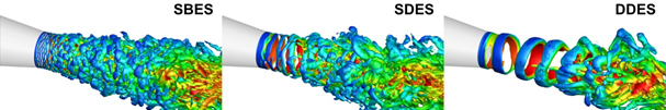
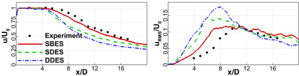
Figure 2.5: Distribution of the Mean (Left) and RMS (Right) Velocity along the Jet Centerline shows the comparison with experimental data. The left plot shows the mean axial velocity along the centerline of the jet; the right plot shows the corresponding streamwise RMS fluctuations. It is clear from both comparisons that the agreement with the data improves with the model’s ability to quickly switch into LES mode.