


Ansys CFX uses an element-based finite volume method, which first involves discretizing the spatial domain using a mesh. The mesh is used to construct finite volumes, which are used to conserve relevant quantities such as mass, momentum, and energy. The mesh is three dimensional, but for simplicity we will illustrate this process for two dimensions.
The figure below shows a typical two-dimensional mesh. All solution variables and fluid properties are stored at the nodes (mesh vertices). A control volume (the shaded area) is constructed around each mesh node using the median dual (defined by lines joining the centers of the edges and element centers surrounding the node).

To illustrate the finite volume methodology, consider the conservation equations for mass, momentum, and a passive scalar, expressed in Cartesian coordinates:
 | (11–1) |
 | (11–2) |
 | (11–3) |
These equations are integrated over each control volume, and Gauss’ Divergence Theorem is applied to convert volume integrals involving divergence and gradient operators to surface integrals. If control volumes do not deform in time, then the time derivatives can be moved outside of the volume integrals and the integrated equations become:
 | (11–4) |
 | (11–5) |
 | (11–6) |
where V and s respectively denote volume and surface regions of integration, and dn j are the differential Cartesian components of the outward normal surface vector. The volume integrals represent source or accumulation terms, and the surface integrals represent the summation of the fluxes. Note that changes to these equations need some generalization to account for mesh deformation. For details, see Mesh Deformation.
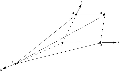
The next step in the numerical algorithm is to discretize the volume and surface integrals. To illustrate this step, consider a single element like the one shown below.
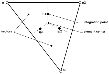
Volume integrals are discretized within each element sector and accumulated to the control volume to which the sector belongs. Surface integrals are discretized at the integration points (ipn) located at the center of each surface segment within an element and then distributed to the adjacent control volumes. Because the surface integrals are equal and opposite for control volumes adjacent to the integration points, the surface integrals are guaranteed to be locally conservative.
After discretizing the volume and surface integrals, the integral equations become:
 | (11–7) |
 | (11–8) |
 | (11–9) |
where  , V is the control volume,
  is the time step,
  is the discrete outward surface vector, the subscript ip denotes evaluation at an integration point, summations
are over all the integration points of the control volume, and the
superscript o refers to the old time level.
Note that the First Order Backward Euler scheme has been assumed in
these equations, although a second order scheme (discussed later)
is usually preferable for transient accuracy.
is the discrete outward surface vector, the subscript ip denotes evaluation at an integration point, summations
are over all the integration points of the control volume, and the
superscript o refers to the old time level.
Note that the First Order Backward Euler scheme has been assumed in
these equations, although a second order scheme (discussed later)
is usually preferable for transient accuracy.
Many discrete approximations developed for CFD are based on series expansion approximations of continuous functions (such as the Taylor series). The order accuracy of the approximation is determined by the exponent on the mesh spacing or time step factor of the largest term in the truncated part of the series expansion, which is the first term excluded from the approximation. Increasing the order-accuracy of an approximation generally implies that errors are reduced more quickly with mesh or time step size refinement. Unfortunately, in addition to increasing the computational load, high-order approximations are also generally less robust (that is, less numerically stable) than their low-order counterparts. Ansys CFX uses second order accurate approximations as much as possible. The role of error is discussed further in Discretization Errors.
Solution fields and other properties are stored at the mesh
nodes. However, to evaluate many of the terms, the solution field
or solution gradients must be approximated at integration points. Ansys CFX uses
finite-element shape functions (unless otherwise noted) to perform
these approximations. Finite-element shape functions describe the
variation of a variable  varies within an element as follows:
 | (11–10) |
where N
i is the
shape function for node i and  is the value of
  at node i. The summation is over all nodes of an element. Key
properties of shape functions include:
at node i. The summation is over all nodes of an element. Key
properties of shape functions include:
 | (11–11) |
 | (11–12) |
The shape functions used in Ansys CFX are linear in terms of parametric coordinates. They are used to calculate various geometric quantities as well, including ip coordinates and surface area vectors. This is possible because Equation 11–10 also holds for the coordinates:
 | (11–13) |
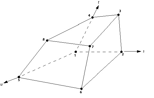
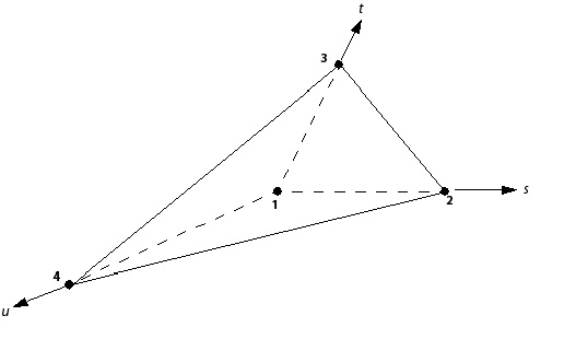
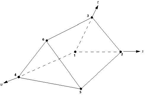
The tri-linear shape functions for each supported mesh element are given below:


In a few situations, gradients are required at nodes. Ansys CFX uses a form of the Gauss’ divergence theorem to evaluate these control volume gradients:
 | (11–18) |
where  is the outward surface vector at ip.
This formula requires that  be evaluated
at integration points using finite-element shape functions.
be evaluated
at integration points using finite-element shape functions.
The advection term requires the integration point values of  to
be approximated in terms of the nodal values of
to
be approximated in terms of the nodal values of  . The advection
schemes implemented in Ansys CFX can be cast in the form:
. The advection
schemes implemented in Ansys CFX can be cast in the form:
 | (11–19) |
where  is the value at the upwind node, and
  is the vector
from the upwind node to the ip. Particular choices
for
is the vector
from the upwind node to the ip. Particular choices
for  and
and  yield different schemes as described below.
A value of  yields a first order Upwind Difference
Scheme (UDS). This scheme is very robust, but it will introduce diffusive
discretization errors that tend to smear steep spatial gradients as
shown below:
yields a first order Upwind Difference
Scheme (UDS). This scheme is very robust, but it will introduce diffusive
discretization errors that tend to smear steep spatial gradients as
shown below:

By choosing a value for  between 0 and 1, and by setting
  equal to the average of the adjacent nodal gradients,
the discretization errors associated with the UDS are reduced. The
quantity
equal to the average of the adjacent nodal gradients,
the discretization errors associated with the UDS are reduced. The
quantity  , called
the Numerical Advection Correction, may be viewed as an anti-diffusive
correction applied to the upwind scheme. The choice
, called
the Numerical Advection Correction, may be viewed as an anti-diffusive
correction applied to the upwind scheme. The choice  is formally
second-order-accurate in space, and the resulting discretization will
more accurately reproduce steep spatial gradients than first order
UDS. However, it is unbounded, and may introduce dispersive discretization
errors that tend to cause non-physical oscillations in regions of
rapid solution variation as shown below.
is formally
second-order-accurate in space, and the resulting discretization will
more accurately reproduce steep spatial gradients than first order
UDS. However, it is unbounded, and may introduce dispersive discretization
errors that tend to cause non-physical oscillations in regions of
rapid solution variation as shown below.

With the central difference scheme (CDS),  is set to
1 and
is set to
1 and  is set to
the local element gradient. An alternative interpretation is that
is set to
the local element gradient. An alternative interpretation is that  is evaluated using the tri-linear shape
functions:
is evaluated using the tri-linear shape
functions:
 | (11–20) |
The resulting scheme is also second-order-accurate, and shares the unbounded and dispersive properties of the Specified Blend Factor scheme. An additional undesirable attribute is that CDS may suffer from serious decoupling issues. While use of this scheme is not generally recommended, it has proven both useful for LES-based turbulence models.
The central differencing scheme described above is an ideal choice in view of its low numerical diffusion. However, it often leads to unphysical oscillations in the solution fields. In order to avoid these oscillations, the bounded central difference (BCD) scheme can be used as the advection scheme.
The bounded central difference scheme is essentially based on the normalized variable diagram (NVD) approach [213] together with the convection boundedness criterion (CBC) [214]. It uses the central difference scheme wherever possible, but blends to the first-order upwind scheme when the CBC is violated.
The bounded central difference scheme is suitable both for the LES and the SAS or DES turbulence models. For SAS and DES, the bounded central difference scheme then replaces the numerical blending between the central differencing scheme and the specified differencing scheme. See Discretization of the Advection Terms for more details regarding the numerical blending.
The High Resolution Scheme uses a special nonlinear recipe for  at
each node, computed to be as close to 1 as possible without introducing
new extrema. The advective flux is then evaluated using the values
of
at
each node, computed to be as close to 1 as possible without introducing
new extrema. The advective flux is then evaluated using the values
of  and
and  from the upwind node. The recipe for
  is
based on the boundedness principles used by Barth and Jesperson [28]. This methodology
involves first computing a
is
based on the boundedness principles used by Barth and Jesperson [28]. This methodology
involves first computing a  and
and  at each node using a stencil involving adjacent
nodes (including the node itself). Next, for each integration point
around the node, the following equation is solved for
at each node using a stencil involving adjacent
nodes (including the node itself). Next, for each integration point
around the node, the following equation is solved for  to
ensure that it does not undershoot
to
ensure that it does not undershoot  or overshoot
  :
:
 | (11–21) |
The nodal value for  is taken to be the minimum value
of all integration point values surrounding the node. The value of
is taken to be the minimum value
of all integration point values surrounding the node. The value of  is
also not permitted to exceed 1. This algorithm can be shown to be
Total Variation Diminishing (TVD) when applied to one-dimensional
situations.
is
also not permitted to exceed 1. This algorithm can be shown to be
Total Variation Diminishing (TVD) when applied to one-dimensional
situations.
Following the standard finite-element approach, shape functions are used to evaluate spatial derivatives for all the diffusion terms. For example, for a derivative in the X direction at integration point ip:
 | (11–22) |
The summation is over all the shape functions for the element. The Cartesian derivatives of the shape functions can be expressed in terms of their local derivatives via the Jacobian transformation matrix:
 | (11–23) |
The shape function gradients can be evaluated at the actual location of each integration point (that is, true tri-linear interpolation), or at the location where each ip surface intersects the element edge (that is, linear-linear interpolation). The latter formulation improves solution robustness at the expense of locally reducing the spatial order-accuracy of the discrete approximation.
The surface integration of the pressure gradient in the momentum equations involves evaluation of the expression:
 | (11–24) |
The value of P ip is evaluated using the shape functions:
 | (11–25) |
As with the diffusion terms, the shape function used to interpolate  can be evaluated
at the actual location of each integration point (that is, true tri-linear
interpolation), or at the location where each ip surface intersects
the element edge (that is, linear-linear interpolation). By default,
linear-linear interpolation is used unless the flow involves buoyancy,
in which case tri-linear interpolation is used for improved accuracy.
can be evaluated
at the actual location of each integration point (that is, true tri-linear
interpolation), or at the location where each ip surface intersects
the element edge (that is, linear-linear interpolation). By default,
linear-linear interpolation is used unless the flow involves buoyancy,
in which case tri-linear interpolation is used for improved accuracy.
The discrete mass flow through a surface of the control volume,
denoted by  , is given by:
 | (11–26) |
This expression must be discretized carefully to lead to proper pressure-velocity coupling and to accurately handle the effects of compressibility, as discussed below.
Ansys CFX uses a co-located (non-staggered) grid layout such that the control volumes are identical for all transport equations. As discussed by Patankar [118], however, naïve co-located methods lead to a decoupled (checkerboard) pressure field. Rhie and Chow [2] proposed an alternative discretization for the mass flows to avoid the decoupling, and this discretization was modified by Majumdar [119] to remove the dependence of the steady-state solution on the time step.
A similar strategy is adopted in Ansys CFX. By applying a momentum-like equation to each integration point, the following expression for the advecting (mass-carrying) velocity at each integration point is obtained:
 | (11–27) |
 | (11–28) |
 | (11–29) |
 = approximation to the central
coefficient of momentum equation, excluding the transient term
= approximation to the central
coefficient of momentum equation, excluding the transient term
 | (11–30) |
The overbars indicate averaging of adjacent vertex values to the integration point, while the o superscript denotes values at the previous time step.
The naïve discretization, given simply by averaging the adjacent vertex velocities to the integration point, is augmented by a high-order pressure variation that scales with the mesh spacing. In particular, when substituted into the continuity equation, the expression
 | (11–31) |
becomes a fourth derivative of pressure that scales with  . This expression represents a spatially third-order
accurate term, and is sometimes also called the pressure-redistribution
term. This term is usually significantly smaller than the average
of vertex velocities, especially as the mesh is refined to reasonable
levels.
. This expression represents a spatially third-order
accurate term, and is sometimes also called the pressure-redistribution
term. This term is usually significantly smaller than the average
of vertex velocities, especially as the mesh is refined to reasonable
levels.
In some cases, the pressure-redistribution term can produce
apparently significant spurious velocity fields. This may occur when
a strong pressure gradient is required to balance a body force,  , such as buoyancy or porous drag. In these cases,
the Rhie Chow discretization may lead to velocity wiggles at locations
where the body force is discontinuous (for example., at a free surface
interface, or at the boundary of a porous region). The wiggles are
greatly reduced or eliminated by redistributing the body force as
follows:
, such as buoyancy or porous drag. In these cases,
the Rhie Chow discretization may lead to velocity wiggles at locations
where the body force is discontinuous (for example., at a free surface
interface, or at the boundary of a porous region). The wiggles are
greatly reduced or eliminated by redistributing the body force as
follows:
 | (11–32) |
Mass flow terms in the mass conservation equation involve a product of the density and the advecting velocity. For compressible flows, the discretization of this product is made as implicit as possible with the use of the following Newton-Raphson linearization:
 | (11–33) |
Here, the superscripts  and
and  respectively indicate
the current and previous iterates. This results in an active linearization
involving both the new density and velocity terms for compressible
flows at any Mach number. The value of
respectively indicate
the current and previous iterates. This results in an active linearization
involving both the new density and velocity terms for compressible
flows at any Mach number. The value of  is linearized in terms of pressure as
 | (11–34) |
For control volumes that do not deform in time, the general discrete approximation of the transient term for the nth time step is:
 | (11–35) |
where values at the start and end of the time step are assigned the superscripts n+½ and n-½, respectively.
With the First Order Backward Euler scheme, the start and end of time step values are respectively approximated using the old and current time level solution values. The resulting discretization is:
 | (11–36) |
It is robust, fully implicit, bounded, conservative in time, and does not have a time step size limitation. This discretization is, however, only first-order accurate in time and will introduce discretization errors that tend to diffuse steep temporal gradients. This behavior is similar to the numerical diffusion experienced with the Upwind Difference Scheme for discretizing the advection term.
With the Second Order Backward Euler scheme, the start and end of time step values are respectively approximated as:
 | (11–37) |
 | (11–38) |
When these values are substituted into the general discrete approximation, Equation 11–35, the resulting discretization is:
 | (11–39) |
This scheme is also robust, implicit, conservative in time, and does not have a time step size limitation. It is second-order accurate in time, but is not bounded and may create some nonphysical solution oscillations. For quantities such as volume fractions, where boundedness is important, a modified Second Order Backward Euler scheme is used instead.
The default startup option for 2nd order transient discretization
uses 1st order discretization for the first timestep. Since 1st order
discretization interprets the solution at the end of the timestep,
and 2nd order discretization interprets the solution in the middle
of the timestep, a conservation error occurs in the first step. The
expert parameter transient startup option (described
in Discretization Parameters in the CFX-Solver Modeling Guide) can be used to partially correct this 'half-timestep' conservation
error. The error can be further minimized by reducing the timestep.
The integral conservation equations presented above in Equation 11–4 must be modified when the control volumes deform in time. These modifications follow from the application of the Leibnitz Rule:
 | (11–40) |
where  is the velocity of
the control volume boundary.
is the velocity of
the control volume boundary.
As before, the differential conservation equations are integrated over a given control volume. At this juncture, the Leibnitz Rule is applied, and the integral conservation equations become:
 | (11–41) |
 | (11–42) |
 | (11–43) |
The transient term accounts for the rate of change of storage in the deforming control volume, and the advection term accounts for the net advective transport across the control volume's moving boundaries.
Erroneous sources of conserved quantities will result if the Geometric Conservation Law (GCL):
 | (11–44) |
is not satisfied by the discretized transient and advection terms. The GCL simply states that for each control volume, the rate of change of volume must exactly balance the net volume swept due to the motion of its boundaries. The GCL is satisfied by using the same volume recipes for both the control volume and swept volume calculations, rather than by approximating the swept volumes using the mesh velocities.