


The CFX-Solver Output file is a formatted text file generated by the CFX-Solver and contains information about your CFX model setup, the state of the solution during execution of the CFX-Solver, and analysis statistics for the particular run. This is the same information written to the text output window of the CFX-Solver Manager. For details, see Text Output Window.
The file is formatted and divided into sections to enable quick and easy interpretation. The sections that are present for any calculation may depend upon which physical models are being used (that is, whether the model is transient or steady-state) and whether the CFX-Solver is being run as several parallel processes or as a single process.
The CFX-Solver will generate a CFX-Solver Output file with a name based on the CFX-Solver Input
file. For example, running the CFX-Solver using the input file named
file.def in a clean working directory will generate a
CFX-Solver Output file named file_001.out.
The header is written at the start of every CFX-Solver Output file and contains information regarding the command that started the job. This information is used to check which files were used to start the run.
The CFX Command Language section describes the problem definition, including domain specification, boundary conditions, meshing parameters and solver control.
The section for the command file looks similar to the following:
 +--------------------------------------------------------------------+
 |                                                                    |
 |                    CFX Command Language for Run                    |
 |                                                                    |
 +--------------------------------------------------------------------+

 LIBRARY:
   MATERIAL: Water
     Material Description = Water (liquid)
     Material Group = Water Data, Constant Property Liquids
     Option = Pure Substance
     Thermodynamic State = Liquid
     PROPERTIES:
       Option = General Material
       EQUATION OF STATE:
         Density = 997.0 [kg m^-3]
         Molar Mass = 18.02 [kg kmol^-1]
         Option = Value
       END
       SPECIFIC HEAT CAPACITY:
         Option = Value
         Specific Heat Capacity = 4181.7 [J kg^-1 K^-1]
         Specific Heat Type = Constant Pressure
       END
       REFERENCE STATE:
         Option = Specified Point
         Reference Pressure = 1 [atm]
         Reference Specific Enthalpy = 0.0 [J/kg]
         Reference Specific Entropy = 0.0 [J/kg/K]
         Reference Temperature = 25 [C]
       END
       DYNAMIC VISCOSITY:
         Dynamic Viscosity = 8.899E-4 [kg m^-1 s^-1]
         Option = Value
       END
       THERMAL CONDUCTIVITY:
         Option = Value
         Thermal Conductivity = 0.6069 [W m^-1 K^-1]
       END
       ABSORPTION COEFFICIENT:
         Absorption Coefficient = 1.0 [m^-1]
         Option = Value
       END
       SCATTERING COEFFICIENT:
         Option = Value
         Scattering Coefficient = 0.0 [m^-1]
       END
       REFRACTIVE INDEX:
         Option = Value
         Refractive Index = 1.0 [m m^-1]
       END
       THERMAL EXPANSIVITY:
         Option = Value
         Thermal Expansivity = 2.57E-04 [K^-1]
       END
     END
   END
 END
 FLOW: Flow Analysis 1
   SOLUTION UNITS:
     Angle Units = [rad]
     Length Units = [m]
     Mass Units = [kg]
     Solid Angle Units = [sr]
     Temperature Units = [K]
     Time Units = [s]
   END
   ANALYSIS TYPE:
     Option = Steady State
     EXTERNAL SOLVER COUPLING:
       Option = None
     END
   END
   DOMAIN: Default Domain
     Coord Frame = Coord 0
     Domain Type = Fluid
     Location = B1.P3
     BOUNDARY: Default Domain Default
       Boundary Type = WALL
       Location = F1.B1.P3,F2.B1.P3,F4.B1.P3,F5.B1.P3,F6.B1.P3,F8.B1.P3
       BOUNDARY CONDITIONS:
         HEAT TRANSFER:
           Option = Adiabatic
         END
         MASS AND MOMENTUM:
           Option = No Slip Wall
         END
         WALL ROUGHNESS:
           Option = Smooth Wall
         END
       END
     END
     BOUNDARY: in1
       Boundary Type = INLET
       Location = in1
       BOUNDARY CONDITIONS:
         FLOW REGIME:
           Option = Subsonic
         END
         HEAT TRANSFER:
           Option = Static Temperature
           Static Temperature = 315 [K]
         END
         MASS AND MOMENTUM:
           Normal Speed = 2 [m s^-1]
           Option = Normal Speed
         END
         TURBULENCE:
           Option = Medium Intensity and Eddy Viscosity Ratio
         END
       END
     END
     BOUNDARY: in2
       Boundary Type = INLET
       Location = in2
       BOUNDARY CONDITIONS:
         FLOW REGIME:
           Option = Subsonic
         END
         HEAT TRANSFER:
           Option = Static Temperature
           Static Temperature = 285 [K]
         END
         MASS AND MOMENTUM:
           Normal Speed = 2 [m s^-1]
           Option = Normal Speed
         END
         TURBULENCE:
           Option = Medium Intensity and Eddy Viscosity Ratio
         END
       END
     END
     BOUNDARY: out
       Boundary Type = OUTLET
       Location = out
       BOUNDARY CONDITIONS:
         FLOW REGIME:
           Option = Subsonic
         END
         MASS AND MOMENTUM:
           Option = Average Static Pressure
           Pressure Profile Blend = 0.05
           Relative Pressure = 0 [Pa]
         END
         PRESSURE AVERAGING:
           Option = Average Over Whole Outlet
         END
       END
     END
     DOMAIN MODELS:
       BUOYANCY MODEL:
         Option = Non Buoyant
       END
       DOMAIN MOTION:
         Option = Stationary
       END
       MESH DEFORMATION:
         Option = None
       END
       REFERENCE PRESSURE:
         Reference Pressure = 1 [atm]
       END
     END
     FLUID DEFINITION: Water
       Material = Water
       Option = Material Library
       MORPHOLOGY:
         Option = Continuous Fluid
       END
     END
     FLUID MODELS:
       COMBUSTION MODEL:
         Option = None
       END
       HEAT TRANSFER MODEL:
         Option = Thermal Energy
       END
       THERMAL RADIATION MODEL:
         Option = None
       END
       TURBULENCE MODEL:
         Option = k epsilon
       END
       TURBULENT WALL FUNCTIONS:
         Option = Scalable
       END
     END
   END
   OUTPUT CONTROL:
     RESULTS:
       File Compression Level = Default
       Option = Standard
     END
   END
   SOLVER CONTROL:
     Turbulence Numerics = First Order
     ADVECTION SCHEME:
       Option = Upwind
     END
     CONVERGENCE CONTROL:
       Maximum Number of Iterations = 100
       Minimum Number of Iterations = 1
       Physical Timescale = 2 [s]
       Timescale Control = Physical Timescale
     END
     CONVERGENCE CRITERIA:
       Residual Target = 1.E-4
       Residual Type = RMS
     END
     DYNAMIC MODEL CONTROL:
       Global Dynamic Model Control = On
     END
   END
 END
 COMMAND FILE:
   Version = 12.0.1
   Results Version = 12.0
 END
 SIMULATION CONTROL:
   EXECUTION CONTROL:
     INTERPOLATOR STEP CONTROL:
       Runtime Priority = Standard
       EXECUTABLE SELECTION:
         Double Precision = Off
       END
     END
     PARALLEL HOST LIBRARY:
       HOST DEFINITION: computer123
         Host Architecture String = winnt-amd64
         Installation Root = D:\Program Files\ANSYS Inc\v%v\CFX
       END
     END
     PARTITIONER STEP CONTROL:
       Multidomain Option = Independent Partitioning
       Runtime Priority = Standard
       EXECUTABLE SELECTION:
         Use Large Problem Partitioner = Off
       END
       PARTITIONING TYPE:
         MeTiS Type = k-way
         Option = MeTiS
         Partition Size Rule = Automatic
       END
     END
     RUN DEFINITION:
       Run Mode = Full
       Solver Input File = \
         D:\examples\StaticMixer.def
     END
     SOLVER STEP CONTROL:
       Runtime Priority = Standard
       EXECUTABLE SELECTION:
         Double Precision = Off
       END
       PARALLEL ENVIRONMENT:
         Number of Processes = 1
         Start Method = Serial
       END
     END
   END
 END
This section describes the job characteristics in terms of the Run mode (sequential or parallel), the machine on which the job was started, and the time and date of the start of the run.
The section for job information for a serial run looks similar to the following:
 +--------------------------------------------------------------------+
 |                  Job Information at Start of Run                   |
 +--------------------------------------------------------------------+

 Run mode:       serial run

 Host computer:  host1 (PID:29363)

 Job started:    Fri Nov 29 17:01:29 2013
Note: The amount of memory required might be more or less than the initial memory allocation amount reported near the start of the run. 1 word is usually 4 bytes, 1 Mword = 1000000 words, and 1 Mbyte = 1048576 bytes.
The section for memory usage looks similar to the following:
 +--------------------------------------------------------------------+
 |         Initial Memory Allocation  (Actual usage may vary)         |
 +--------------------------------------------------------------------+
 |         | Real       | Integer    | Character |  Logical | Double  |
 ----------+------------+------------+-----------+----------+----------
 | Mwords  | 8.69       | 2.05       | 7.87      | 0.12     | 0.09    |
 | Mbytes  | 33.15      | 7.82       | 7.51      | 0.46     | 0.69    |
 ----------+------------+------------+-----------+----------+----------
 +--------------------------------------------------------------------+
 |            Host Memory Information (Mbytes): Solver                |
 +--------------------------------------------------------------------+
 |          Host           |     System     |   Allocated    |   %    |
 +-------------------------+----------------+----------------+--------+
 | fastcomputer1           |     65293.18   |        49.62   |   0.08 |
 +-------------------------+----------------+----------------+--------+
The peak memory usage over the lifetime of the run is reported near the end of the run. For example:
 +--------------------------------------------------------------------+
 |            Host Memory Information (Mbytes): Solver                |
 +--------------------------------------------------------------------+
 |          Host           |     System     |      Peak      |   %    |
 +-------------------------+----------------+----------------+--------+
 | fastcomputer1           |     65293.18   |        65.72   |   0.10 |
 +-------------------------+----------------+----------------+--------+
If the Maximal memory allocation option is used,
the controlling parameters are also reported. For example:
 +--------------------------------------------------------------------+
 |                     Memory Allocation Strategy                     |
 +--------------------------------------------------------------------+

 Up to 80.00 % of the system memory will be used, within lower and
 upper bounds of 1.00 and 10.00 times the estimated memory.


 +--------------------------------------------------------------------+
 |         Initial Memory Allocation  (Actual usage may vary)         |
 +--------------------------------------------------------------------+

           | Real       | Integer    | Character | Logical  | Double
 ----------+------------+------------+-----------+----------+----------
 Mwords    |   18550.27 |    4166.74 |     60.94 |     0.86 |     8.61
 Mbytes    |   70763.67 |   31789.67 |     58.11 |     6.52 |    65.67
 ----------+------------+------------+-----------+----------+----------


 +--------------------------------------------------------------------+
 |            Host Memory Information (Mbytes): Solver                |
 +--------------------------------------------------------------------+
 |          Host           |     System     |   Allocated    |   %    |
 +-------------------------+----------------+----------------+--------+
 | fastcomputer1           |    128354.55   |    102683.65   |  80.00 |
+-------------------------+----------------+----------------+--------+Mesh statistics summarize the following domain-specific and global (across all domains) items:
Mesh quality diagnostics
The total number of nodes, elements and boundary faces in the mesh
The area fractions of mesh interfaces that were unmapped.
Mesh quality diagnostics include measures of mesh orthogonality, expansion and aspect ratio (see Mesh Issues). For each measure, there are value ranges that are considered good, acceptable, and poor (the latter indicating potential accuracy or convergence problems). These ranges are annotated with OK, ok, and !, respectively, in the mesh diagnostics summary. The relevant minimum or maximum value is presented for each measure, plus a summary of the percent of the mesh with values in each of the good, acceptable, and poor ranges. Note that these percentages are rounded to the nearest integer value. In the sample output presented below, the worst expansion factor is 37, which is considered poor (that is, annotated with !). While slightly more than 1% of the impeller mesh exhibits similarly poor values, less than 1% of the global mesh is considered poor and "<1" is written in the summary.
The section for mesh statistics looks similar to the following:
 +--------------------------------------------------------------------+
 |                          Mesh Statistics                           |
 +--------------------------------------------------------------------+
 | Domain Name          | Orthog. Angle | Exp. Factor  | Aspect Ratio |
 +----------------------+---------------+--------------+--------------+
 |                      | Minimum [deg] |   Maximum    |    Maximum   |
 +----------------------+---------------+--------------+--------------+
 | impeller             |       34.7 ok |        37  ! |        13 OK |
 | tank                 |       61.4 OK |        11 ok |       303 OK |
 | Global               |       34.7 ok |        37  ! |       303 OK |
 +----------------------+---------------+--------------+--------------+
 |                      |  %!  %ok  %OK | %!  %ok  %OK | %!  %ok  %OK |
 +----------------------+---------------+--------------+--------------+
 | impe                 |   0   11   89 |  1   32   67 |  0    0  100 |
 | tank                 |   0    0  100 |  0    2   98 |  0    3   97 |
 | Global               |   0    3   97 | <1   11   89 |  0    2   98 |
 +----------------------+---------------+--------------+--------------+

 Domain Name : impeller

     Total Number of Nodes                                =        1710

     Total Number of Elements                             =        7554
         Total Number of Tetrahedrons                     =        7206
         Total Number of Prisms                           =         238
         Total Number of Pyramids                         =         110

     Total Number of Faces                                =        1494

 Domain Name : tank

     Total Number of Nodes                                =        4558

     Total Number of Elements                             =        3610
         Total Number of Hexahedrons                      =        3610

     Total Number of Faces                                =        2212

 Global Statistics :

     Global Number of Nodes                               =        6268

     Global Number of Elements                            =       11164
         Total Number of Tetrahedrons                     =        7206
         Total Number of Prisms                           =         238
         Total Number of Hexahedrons                      =        3610
         Total Number of Pyramids                         =         110

     Global Number of Faces                               =        3706

 Domain Interface Name : ImpellerPeriodic

     Non-overlap area fraction on side 1                  =    0.00E+00
     Non-overlap area fraction on side 2                  =    0.00E+00

 Domain Interface Name : TankPeriodic1 TankPeriodic2

     Non-overlap area fraction on side 1                  =    0.00E+00
     Non-overlap area fraction on side 2                  =    0.00E+00
The mesh quality thresholds that define the OK (good), ok (acceptable), and ! (poor) status in the mesh statistics section of the CFX-Solver Output file are as follows:
| Maximum aspect ratio (double precision) | OK | <10000.0 |
| ok | 10000.0 < 100000.0 | |
| ! | > 100000.0 | |
| Maximum aspect ratio (single precision) | OK | < 100.0 |
| ok | 100.0 < 1000.0 | |
| ! | > 1000.0 | |
| Maximum mesh expansion factor | OK | < 5.0 |
| ok | 5.0 < 20.0 | |
| ! | > 20.0 | |
| Minimum orthogonal angle | OK | > 50° |
| ok | 50° > 20° | |
| ! | < 20° |
Note: Negative orthogonality angles are possible and indicate the presence of very poor mesh elements that can adversely affect solution quality. It is recommended that meshes not contain any negative orthogonality angles.
These are average scales based on the initial flow field. If the initial velocity field is zero, then the initial average velocity scale will also be zero.
The section for initial average scales looks similar to the following:
+--------------------------------------------------------------------+
|                      Average Scale Information                     |
+--------------------------------------------------------------------+
Domain Name : StaticMixer
     Global Length                                       =  3.2113E+00
     Density                                             =  9.9800E+02
     Dynamic Viscosity                                   =  1.0000E-03
     Velocity                                            =  0.0000E+00
     Thermal Conductivity                                =  5.9100E-01
     Specific Heat Capacity at Constant Pressure         =  4.1900E+03
     Prandtl Number                                      =  7.0897E+00
For serial runs, the solver checks to see if any fluid domain contains volumetric regions that are isolated pockets. This check cannot be performed for parallel solver runs.
This section lists the dependent variables solved and the equations to which they relate as well as the estimated physical timestep if calculated automatically.
Equations are given two labels: the individual name and a combined name used for combining residuals together. Residuals for multi-domain problems are combined provided the domains are connected together and have the same domain type (solid or fluid/porous). If there are multiple groups of the same domain type, then the group residual is identified by the name of the first domain in the connected group.
The section for solved equations looks similar to the following:
 +--------------------------------------------------------------------+
 |              The Equations Solved in This Calculation              |
 +--------------------------------------------------------------------+
 Subsystem : Momentum and Mass
   U-Mom
   V-Mom
   W-Mom
   P-Mass
 Subsystem : Thermal Radiation
   I-Radiation
 Subsystem : Heat Transfer
   H-Energy
 Subsystem : Temperature Variance
   T-Variance
 Subsystem : TurbKE and Diss.K
   K-TurbKE
   E-Diss.K
 Subsystem : Mixture Fraction
   Z-Mean
   Z-Variance
 Subsystem : Mass Fractions
   NO-Mass Fraction
The convergence history section details the state of the solution as it progresses. Equation residual information at specified locations enables you to monitor the convergence. Convergence difficulties can often be pinpointed to a particular part of the solution (for example, the momentum equation), and/or a particular location.
The tables shown in the convergence history have the following columns:
The rate is defined as seen in Equation 3–1 where
 is the residual at iteration
  , and
, and  is the residual at an earlier iteration. Rates less
than 1.0 indicate convergence.
is the residual at an earlier iteration. Rates less
than 1.0 indicate convergence.
(3–1)
The value of the root mean square normalized residual taken over the whole domain.
The value of the maximum normalized residual in the domain.
The three columns in this section refer to the performance of the linear (inner) solvers. The first column is the average number of iterations the linear solvers attempted to obtain the specified linear equation convergence criteria (within a specified number of iterations). The second column gives the normalized residuals for the solutions to the linear equation. The last column can have one of four entries:
*indicates that there was a numerical floating point exception and this resulted in the failure of the linear solvers.Findicates that the linear solvers did not reduce the residuals (that is, the solution was diverging), but the linear solvers may carry on if the divergence is not catastrophic.okindicates that the residuals were reduced, but that the degree of reduction did not meet the specified criteria.OKindicates that the specified convergence criteria for the reduction of residuals was achieved.
After the convergence criteria has been achieved, or the specified number of timesteps has been reached, CFX-Solver appends additional information, calculated from the solution, to the CFX-Solver Output file.
The convergence history for a steady state analysis looks similar to the following:
+--------------------------------------------------------------------+
|                       Convergence History                          |
+--------------------------------------------------------------------+
======================================================================
OUTER LOOP ITERATION =    1                     CPU SECONDS = 2.68E+00
----------------------------------------------------------------------
|       Equation       | Rate | RMS Res | Max Res |  Linear Solution |
+----------------------+------+---------+---------+------------------+
| U - Mom              | 0.00 | 1.5E-10 | 5.4E-09 |       1.5E+10  ok|
| V - Mom              | 0.00 | 1.6E-04 | 3.2E-03 |       6.4E+01  ok|
| W - Mom              | 0.00 | 2.5E-10 | 6.4E-09 |       1.1E+10  ok|
| P - Mass             | 0.00 | 2.2E-03 | 3.0E-02 | 12.0  9.5E-02  OK|
+----------------------+------+---------+---------+------------------+
| H-Energy             | 0.00 | 3.6E-03 | 3.6E-02 |  5.4  8.0E-03  OK|
+----------------------+------+---------+---------+------------------+
======================================================================
OUTER LOOP ITERATION =    2                     CPU SECONDS = 1.24E+01
----------------------------------------------------------------------
|       Equation       | Rate | RMS Res | Max Res |  Linear Solution |
+----------------------+------+---------+---------+------------------+
| U - Mom              |99.99 | 5.2E-03 | 7.5E-02 |       4.8E-02  OK|
| V - Mom              |99.76 | 1.6E-02 | 1.6E-01 |       1.4E-02  OK|
| W - Mom              |99.99 | 8.4E-03 | 1.2E-01 |       7.9E-02  OK|
| P - Mass             | 4.26 | 9.3E-03 | 1.3E-01 |  8.3  8.4E-02  OK|
+----------------------+------+---------+---------+------------------+
| H-Energy             | 0.35 | 1.3E-03 | 8.8E-03 |  9.4  2.9E-03  OK|
+----------------------+------+---------+---------+------------------+
................
................
======================================================================
OUTER LOOP ITERATION =   29                     CPU SECONDS = 2.44E+02
----------------------------------------------------------------------
|       Equation       | Rate | RMS Res | Max Res |  Linear Solution |
+----------------------+------+---------+---------+------------------+
| U - Mom              | 0.86 | 7.7E-05 | 3.1E-04 |       5.1E-02  OK|
| V - Mom              | 0.86 | 9.1E-05 | 3.7E-04 |       4.8E-02  OK|
| W - Mom              | 0.86 | 1.9E-05 | 1.6E-04 |       5.0E-02  OK|
| P - Mass             | 0.87 | 3.7E-05 | 1.7E-04 |  8.3  3.0E-02  OK|
+----------------------+------+---------+---------+------------------+
| H-Energy             | 0.86 | 5.7E-06 | 5.5E-05 |  9.5  9.8E-03  OK|
+----------------------+------+---------+---------+------------------+
CFD Solver finished: Wed Oct 25 16:01:48 2000
CFD Solver wall clock seconds: 1.0000E+00
If a steady state analysis is continued, then the outer loop iterations and CPU seconds for the current run are enclosed in parenthesis, as shown below. Values not enclosed in parenthesis are the totals for the overall analysis.
======================================================================
OUTER LOOP ITERATION =   30 (    1) CPU SECONDS = 2.48E+02 ( 3.38E+00)
----------------------------------------------------------------------
|       Equation       | Rate | RMS Res | Max Res |  Linear Solution |
+----------------------+------+---------+---------+------------------+
| U - Mom              | 0.00 | 1.5E-04 | 1.2E-03 |       4.6E-02  OK|
| V - Mom              | 0.00 | 2.1E-04 | 1.2E-03 |       3.8E-02  OK|
| W - Mom              | 0.00 | 1.5E-04 | 2.1E-03 |       1.3E-02  OK|
| P - Mass             | 0.00 | 3.2E-05 | 1.5E-04 |  8.3  3.4E-02  OK|
+----------------------+------+---------+---------+------------------+
| H-Energy             | 0.00 | 7.7E-06 | 8.5E-05 |  9.5  9.1E-03  OK|
+----------------------+------+---------+---------+------------------+
If the Zero Equation model is used to model turbulence, the overall turbulence viscosity is provided.
The section for computed model constants looks similar to the following:
+--------------------------------------------------------------------+
|                      Computed Model Constants                      |
+--------------------------------------------------------------------+
Turbulence viscosity for Turbulence Model 1   = 3.3667E+00
After executing each coefficient iteration and time step (or outer iteration), the solver evaluates all internal termination conditions and user-defined interrupt control conditions. In the event of a termination or interrupt, any of these conditions that are true are reported in the CFX-Solver Output file as outlined below.
 ======================================================================
               Termination and Interrupt Condition Summary
 ======================================================================
CFD Solver: <internal termination condition description>
User: <interrupt condition object name> Global conservation statistics are generated for all transport equations with the exception of turbulence equations, which have special wall treatment. These are good checks for the convergence of a solution. Small values of global imbalance indicate that conservation has essentially been achieved.
The percentage imbalance of a quantity is calculated as:

where " " is taken to be the largest
contribution in all connected domains for the specific group of equations. The
grouping of equations for the purpose of normalization can be different
depending on the case.
" is taken to be the largest
contribution in all connected domains for the specific group of equations. The
grouping of equations for the purpose of normalization can be different
depending on the case.
For single-phase calculations, each equation imbalance is normalized using the largest contribution for that equation subsystem. The exception is the hydrodynamic subsystem, where each momentum equation imbalance is normalized using the largest contribution from all momentum equations, and the continuity equation imbalance is normalized using the largest contribution in all continuity equations.
For Eulerian multiphase cases, the imbalance normalization can be across all phases or within a single phase for any equation, depending on the physics and whether coupled volume fractions are employed. A summary table of how each equation normalization is performed is given below:
|
Equation |
Normalization | |
|---|---|---|
|
Segregated VFs |
Coupled VFs | |
|
Momentum |
All Phases |
All Phases |
|
Energy |
All Phases |
All Phases |
|
Mass |
Each Phase |
All Phases |
|
Mass [a] |
Each Phase |
All Phases |
|
Components |
Each Phase |
Each Phase |
|
Components [b] |
All Phases |
All Phases |
|
Additional Variables |
Each Phase |
Each Phase |
|
Additional Variables [c] |
All Phases |
All Phases |
The section for global conservation statistics looks similar to the following:
 ======================================================================
              Boundary Flow and Total Source Term Summary
 ======================================================================

 +--------------------------------------------------------------------+
 |                               U-Mom                                |
 +--------------------------------------------------------------------+
 Boundary         : CatConv Default                        -9.4754E-01
 Boundary         : Inlet                                   1.6971E+00
 Boundary         : InletSide Side 1                        1.3262E-05
 Boundary         : Outlet                                 -1.0523E+00
 Boundary         : OutletSide Side 1                      -1.7085E-07
 Sub-Domain       : catalyst                                2.6129E-01
 Neg Accumulation : CatConv                                 4.1436E-02
 Domain Interface : InletSide (Side 1)                     -1.1166E-02
 Domain Interface : InletSide (Side 2)                      1.1166E-02
 Domain Interface : OutletSide (Side 1)                    -1.4308E-05
 Domain Interface : OutletSide (Side 2)                     1.4308E-05
                                                           -----------
 Domain Imbalance :                                        -3.6059E-05


 +--------------------------------------------------------------------+
 |                               V-Mom                                |
 +--------------------------------------------------------------------+
 Boundary         : CatConv Default                        -3.3355E-02
 Boundary         : Inlet                                   1.1009E-07
 Boundary         : InletSide Side 1                        7.2564E-06
 Boundary         : Outlet                                 -4.7561E-04
 Boundary         : OutletSide Side 1                       1.9734E-08
 Sub-Domain       : catalyst                                3.4056E-02
 Neg Accumulation : CatConv                                -2.4319E-04
 Domain Interface : InletSide (Side 1)                     -4.7260E-04
 Domain Interface : InletSide (Side 2)                      4.7262E-04
 Domain Interface : OutletSide (Side 1)                     7.5672E-06
 Domain Interface : OutletSide (Side 2)                    -7.5672E-06
                                                           -----------
 Domain Imbalance :                                        -1.0275E-05


 +--------------------------------------------------------------------+
 |                               W-Mom                                |
 +--------------------------------------------------------------------+
 Boundary         : CatConv Default                        -1.1450E+01
 Boundary         : Inlet                                  -1.6971E+00
 Boundary         : InletSide Side 1                        1.3180E-01
 Boundary         : Outlet                                  1.0628E+00
 Boundary         : OutletSide Side 1                      -6.8369E-02
 Sub-Domain       : catalyst                                1.2137E+01
 Neg Accumulation : CatConv                                -1.8195E-01
 Domain Interface : InletSide (Side 1)                      2.2715E+01
 Domain Interface : InletSide (Side 2)                     -2.2592E+01
 Domain Interface : OutletSide (Side 1)                    -1.0548E+01
 Domain Interface : OutletSide (Side 2)                     1.0493E+01
                                                           -----------
 Domain Imbalance :                                         1.4353E-03


 +--------------------------------------------------------------------+
 |                               P-Mass                               |
 +--------------------------------------------------------------------+
 Boundary         : Inlet                                   2.8382E-02
 Boundary         : Outlet                                 -5.6938E-02
 Neg Accumulation : CatConv                                 2.8576E-02
 Domain Interface : InletSide (Side 1)                     -3.0665E-02
 Domain Interface : InletSide (Side 2)                      3.0665E-02
 Domain Interface : OutletSide (Side 1)                     5.6543E-02
 Domain Interface : OutletSide (Side 2)                    -5.6543E-02
                                                           -----------
 Domain Imbalance :                                         2.0828E-05


 +--------------------------------------------------------------------+
 |                            I-Radiation                             |
 +--------------------------------------------------------------------+
 Boundary         : CatConv Default                        -1.4392E+01
 Boundary         : Inlet                                   1.9442E+01
 Boundary         : InletSide Side 1                        3.8307E-01
 Boundary         : Outlet                                 -6.1793E+00
 Boundary         : OutletSide Side 1                      -1.7803E-01
 Domain Src (Neg) : CatConv                                -2.9646E-01
 Domain Src (Pos) : CatConv                                 3.0447E-01
 Domain Interface : InletSide (Side 1)                     -4.6702E+02
 Domain Interface : InletSide (Side 2)                      4.6702E+02
 Domain Interface : OutletSide (Side 1)                    -7.4487E+01
 Domain Interface : OutletSide (Side 2)                     7.4490E+01
                                                           -----------
 Domain Imbalance :                                        -9.0640E-01


 +--------------------------------------------------------------------+
 |                              H-Energy                              |
 +--------------------------------------------------------------------+
 Boundary         : CatConv Default                         1.4284E+01
 Boundary         : Inlet                                   8.6049E+03
 Boundary         : InletSide Side 1                       -3.8344E-01
 Boundary         : Outlet                                 -2.3960E+02
 Boundary         : OutletSide Side 1                       1.7809E-01
 Domain Src (Neg) : CatConv                                -3.0461E-01
 Domain Src (Pos) : CatConv                                 2.9616E-01
 Neg Accumulation : CatConv                                -8.3717E+03
 Domain Interface : InletSide (Side 1)                     -7.6620E+03
 Domain Interface : InletSide (Side 2)                      7.6620E+03
 Domain Interface : OutletSide (Side 1)                     1.3624E+02
 Domain Interface : OutletSide (Side 2)                    -1.3624E+02
                                                           -----------
 Domain Imbalance :                                         7.6699E+00
An example section that shows how the imbalance for each transport equation is normalized:
+--------------------------------------------------------------------+
|                     Normalised Imbalance Summary                   |
+--------------------------------------------------------------------+
|       Equation       |      Maximum Flow     |     Imbalance (%)   |
+--------------------------------------------------------------------+
| U-Mom-Fluid 2        |       6.0270E+02      |       15.9327       |
| V-Mom-Fluid 2        |       6.0270E+02      |        0.0000       |
| W-Mom-Fluid 2        |       6.0270E+02      |        0.0004       |
| U-Mom-Fluid 1        |       6.0270E+02      |      -16.6732       |
| V-Mom-Fluid 1        |       6.0270E+02      |        0.0001       |
| W-Mom-Fluid 1        |       6.0270E+02      |        0.0004       |
| Mass-Fluid 2         |       5.9820E+02      |       16.2942       |
| Mass-Fluid 1         |       5.9820E+02      |      -16.2929       |
+----------------------+-----------------------+---------------------+
+----------------------+-----------------------+---------------------+
| H-Energy-Fluid 2     |       3.7642E+07      |     -136.9703       |
| H-Energy-Fluid 1     |       3.7642E+07      |      -76.2664       |
+----------------------+-----------------------+---------------------+
For more details, see Monitoring and Obtaining Convergence in the CFX-Solver Modeling Guide.
The CFX-Solver calculates the pressure and viscous components of forces on all boundaries specified as walls. The drag force on any wall can be calculated from these values as follows:
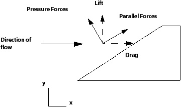
Lift is the net force on the body in the direction perpendicular to the direction of flow. In the above diagram, the lift is the sum of the forces on the wall in the vertical direction, that is, the sum of the pressure force and the viscous force components in the y direction.
Drag is the net force on the body in the direction of the flow. In the above diagram, the drag is the sum of the forces on the wall in the horizontal direction, that is, the sum of the pressure force and the viscous force components in the x direction.
It is apparent from this that viscous force is not a pure shear force because it also has a small component in the normal direction, arising in part from a normal component in the laminar flow shear stress.
The pressure and viscous moments are related to the pressure and viscous
forces calculated at the wall. The pressure moment is the vector product of the
pressure force vector  and
the position vector
and
the position vector  . The viscous moment is the vector
product of the viscous force vector
. The viscous moment is the vector
product of the viscous force vector and
the position vector
and
the position vector  . As an example, review Equation 3–2 where
  and
and  are the pressure and viscous moments respectively.
 | (3–2) |
These are summed over all the surface elements in the wall.
It is important to note that forces are evaluated in the local reference frame
and that they do not include reference pressure effects. The pressure force is
calculated as the integral of the relative pressure over the wall area and not
as the integral of the sum of the reference and relative pressures. You can
include reference pressure effects in the force calculation by setting the
expert parameter
include pref in forces = t.
It is also important to note that for rotating domains in a transient run, forces are evaluated in the reference frame fixed to the initial domain orientation. These quantities are not influenced by any rotation that might occur during a transient run or when a rotational offset is specified. However, results for rotating domains in a transient run may be in the rotated position (depending on the setting of Options in CFD-Post) when they are subsequently loaded into CFD-Post for post-processing.
The sections for calculated wall forces and moments look similar to the following:
 ======================================================================
                     Wall Force and Moment Summary
 ======================================================================

 Notes:
 1. Pressure integrals exclude the reference pressure.  To include
    it, set the expert parameter 'include pref in forces = t'.


 +--------------------------------------------------------------------+
 |                      Pressure Force On Walls                       |
 +--------------------------------------------------------------------+
                                    X-Comp.      Y-Comp.      Z-Comp.

 Domain Group: Bottom Box

 Copy of Walls                    7.5841E+01   8.4350E+01  -5.2096E+02
 Top Box Default                 -5.4841E+01   0.0000E+00   0.0000E+00
 Walls                            4.8468E+01   1.2755E+02   5.0230E+02
                                  -----------  -----------  -----------
 Domain Group Totals :            6.9468E+01   2.1190E+02  -1.8659E+01


 +--------------------------------------------------------------------+
 |                       Viscous Force On Walls                       |
 +--------------------------------------------------------------------+
                                    X-Comp.      Y-Comp.      Z-Comp.

 Domain Group: Bottom Box

 Copy of Walls                   -3.4280E-04  -1.8638E-03  -5.7310E-04
 Top Box Default                 -4.7982E-05   5.5391E-06  -2.2129E-05
 Walls                            2.9180E-04  -4.3111E-05  -6.2137E-04
                                  -----------  -----------  -----------
 Domain Group Totals :           -9.8980E-05  -1.9014E-03  -1.2166E-03
The locations of the maximum residuals are very important when identifying and/or quantifying the root cause of solution convergence difficulties. If there is trouble converging to a steady-state solution and the maximum residuals are large, take the following steps:
In the CFX-Solver Output file, identify the equation that has the largest maximum (not RMS) residuals in the diagnostics section for the final iteration (see Convergence History). Specifically, look at the momentum, mass, and energy equations’ maximum residuals.
Find the
Locations of Maximum Residualstable near the bottom of the CFX-Solver Output file, and identify the domain and node number for the equation with the largest maximum residual.Create a point locator in CFD-Post using the domain and node number identified above by setting Geometry > Method to
Node Number. For details, see Point: Geometry Tab in the CFD-Post User's Guide.
The sections for maximum residual statistics look similar to the following:
 +--------------------------------------------------------------------+
 |               Locations of Maximum Residuals                       |
 +--------------------------------------------------------------------+
 |       Equation       |      Domain Name      |     Node Number     |
 +--------------------------------------------------------------------+
 | U-Mom                | Domain 1              |              34     |
 | V-Mom                | Domain 1              |               4     |
 | W-Mom                | Domain 2              |              61     |
 | P-Mass               | Domain 1              |              61     |
 +----------------------+-----------------------+---------------------+
 | H-Energy             | Domain 2              |              61     |
 +----------------------+-----------------------+---------------------+
 | H2O-Mass Fraction    | Domain 1              |              57     |
 | C2H6O-Mass Fraction  | Domain 1              |               1     |
 | C10H22-Mass Fraction | Domain 2              |              61     |
 +----------------------+-----------------------+---------------------+
The presence of regions of low mesh quality is the most common cause of stalled convergence. A common cause of stalled convergence within steady-state simulations is the presence of recirculating flow or local flow separation. Try to correlate the cause of stalled convergence to the location of the maximum residual in CFD-Post. Check for poor mesh quality, separating flow, reattaching flow, etc. in this location to determine whether the lack of tight convergence is caused by a problem that can be solved (for example, by improving the mesh in this region), or caused by a tolerable oscillation (for example, if some transient flow phenomena is being resolved in an otherwise steady-state flow simulation).
This is only applicable to steady-state simulations (serial and parallel). The
information is equation based, that is there is one line per equation solved.
For each equation, the type of timestepping used is displayed as
Auto, Physical or
Local.
Both Auto and Physical run as false
transients. This means that although the simulation is steady state, a transient
term with an associated timestep is used to relax the equations during
convergence. In this case, the total elapsed pseudo-time is also printed.
The section for false transient information looks similar to the following:
+--------------------------------------------------------------------+
|                   False Transient Information                      |
+--------------------------------------------------------------------+
|       Equation       |       Type        |   Elapsed Pseudo-Time   |
+--------------------------------------------------------------------+
| U - Mom              | Physical          |      5.80000E+01        |
| V - Mom              | Physical          |      5.80000E+01        |
| W - Mom              | Physical          |      5.80000E+01        |
| P - Mass             | Physical          |      5.80000E+01        |
| H-Energy             | Physical          |      5.80000E+01        |
+--------------------------------------------------------------------+
These are average scales for the final flow field.
The section for final average scales looks similar to the following:
+--------------------------------------------------------------------+
|                     Average Scale Information                      |
+--------------------------------------------------------------------+
Domain Name : StaticMixer
	Global Length                                       =  3.2113E+00
	Density                                             =  9.9800E+02
	Dynamic Viscosity                                   =  1.0000E-03
	Velocity                                            =  1.4534E+00
	Advection Time                                      =  2.2095E+00
	Reynolds Number                                     =  4.6581E+06
	Thermal Conductivity                                =  5.9100E-01
	Specific Heat Capacity at Constant Pressure         =  4.1900E+03
	Prandtl Number                                      =  7.0897E+00
	Temperature Range                                   =  3.0008E+01
These are the maximum and minimum values for each variable in the flow field.
The section for variable range information looks similar to the following:
+--------------------------------------------------------------------+
|                     Variable Range Information                     |
+--------------------------------------------------------------------+
Domain Name : StaticMixer
+--------------------------------------------------------------------+
|      Variable Name                         |    min    |    max    |
+--------------------------------------------------------------------+
| Velocity u                                 | -1.65E+00 |  1.61E+00 |
| Velocity v                                 | -2.26E+00 |  2.25E+00 |
| Velocity w                                 | -4.13E+00 |  2.58E-01 |
| Pressure                                   | -6.71E+02 |  1.38E+04 |
| Density                                    |  9.98E+02 |  9.98E+02 |
| Dynamic Viscosity                          |  1.00E-03 |  1.00E-03 |
| Specific Heat Capacity at Constant Pressure|  4.19E+03 |  4.19E+03 |
| Thermal Conductivity                       |  5.91E-01 |  5.91E-01 |
| Thermal Expansivity                        |  2.10E-04 |  2.10E-04 |
| Eddy Viscosity                             |  1.89E+01 |  1.89E+01 |
| Temperature                                |  2.85E+02 |  3.15E+02 |
| Static Enthalpy                            |  1.19E+06 |  1.32E+06 |
+--------------------------------------------------------------------+
The section for CPU requirements looks similar to the following:
 +--------------------------------------------------------------------+
 |           CPU Requirements of Numerical Solution - Total           |
 +--------------------------------------------------------------------+

 Subsystem Name                  Discretization       Linear Solution
                                (secs.   %total)     (secs.   %total)
 ----------------------------------------------------------------------
 Momentum and Mass              2.50E-01  10.5 %     7.81E-02   3.3 %
                                -------- -------     --------  ------
 Subsystem Summary              2.50E-01  10.5 %     7.81E-02   3.3 %

 Variable Updates               1.25E-01   5.3 %
 File Reading                   1.41E-01   5.9 %
 File Writing                   6.25E-02   2.6 %
 Miscellaneous                  1.72E+00  72.4 %
                                --------
 Total                          2.38E+00
The section for job information looks similar to the following:
 +--------------------------------------------------------------------+
 |                   Job Information at End of Run                    |
 +--------------------------------------------------------------------+
 Job finished:   Wed Jul 29 11:28:47 2020
 Total wall clock time: 8.810E+00 seconds
             or: (          0:         0:         0:     8.810 )
                 (       Days:     Hours:   Minutes:   Seconds )