


Engineering turbulence transition predictions are based mainly on two modeling concepts. The first is the use of low-Reynolds number turbulence models, where the wall damping functions of the underlying turbulence model trigger turbulent transition onset. This concept is attractive because it is based on transport equations and can therefore be implemented without much effort. However, experience has shown that this approach is not capable of reliably capturing the influence of the many different factors that affect transition, such as free-stream turbulence, pressure gradients and separation.
The second approach is the use of experimental correlations.
The correlations usually relate the turbulence intensity,  , in the free-stream to the momentum-thickness Reynolds number,
  , at transition onset. Ansys
has developed a locally formulated transport equation for intermittency,
which can be used to trigger transition. The full laminar-turbulent transition model is based on
two transport equations, one for the intermittency and one for the
transition onset criteria in terms of momentum thickness Reynolds
number. It is called the Gamma Theta model and is
the recommended transition model for general-purpose applications.
It uses an empirical correlation (Langtry and Menter) that has
been developed to cover standard bypass transition as well as flows
in low free-stream turbulence environments. This built-in correlation
has been extensively validated together with the SST turbulence model
for a wide range of transitional flows. The transition model can also
be used with the BSL or SAS-SST turbulence models. A description
of the full Gamma Theta model can be found in Two Equation Gamma Theta Transition Model in the CFX-Solver Theory Guide.
, at transition onset. Ansys
has developed a locally formulated transport equation for intermittency,
which can be used to trigger transition. The full laminar-turbulent transition model is based on
two transport equations, one for the intermittency and one for the
transition onset criteria in terms of momentum thickness Reynolds
number. It is called the Gamma Theta model and is
the recommended transition model for general-purpose applications.
It uses an empirical correlation (Langtry and Menter) that has
been developed to cover standard bypass transition as well as flows
in low free-stream turbulence environments. This built-in correlation
has been extensively validated together with the SST turbulence model
for a wide range of transitional flows. The transition model can also
be used with the BSL or SAS-SST turbulence models. A description
of the full Gamma Theta model can be found in Two Equation Gamma Theta Transition Model in the CFX-Solver Theory Guide.
In addition, a very powerful option has been included to enable you to enter your own user defined empirical correlation together with the Gamma Theta model, which can then be used to control the transition onset momentum thickness Reynolds number equation. The method is driven by CCL and as a result any valid CCL expression can be used to define the correlation. A simple example is shown below where the transition Reynolds number was specified as a function of the x-coordinate:
FLUID MODELS:
   TURBULENCE MODEL :
      Option = SST
      TRANSITIONAL TURBULENCE :
         Option = Gamma Theta Model
         TRANSITION ONSET CORRELATION:
            Option = User Defined
            Transition Onset Reynolds Number = 260.0*(1.0 + x/(1.0 [m]))
         END
       END
   END
END
Besides the two-equation Gamma Theta transition model, other reduced models are available:
Specified Intermittency
A zero-equation model, where you can prescribe the intermittency directly as a CEL expression.
The best way to specify the intermittency is with a user defined subroutine that is based on the x, y and z coordinates. This way, conditional statements can be used to define geometric bounds where the intermittency can be specified as zero (laminar flow) or one (turbulent flow). This method can be used to prescribe laminar regions at the leading edges of the wings, for example.
Gamma Model
A one-equation model that solves only the intermittency equation (of the two-equation Gamma Theta transition model) using a user specified value of the transition onset momentum thickness-based Reynolds number.
Intermittency Model
A one-equation model. For details, see One Equation Intermittency Transition Model in the CFX-Solver Theory Guide.
Note:
The Gamma Theta transition model is not Galilean invariant and should therefore not be applied (unless with caution) to walls that move relative to the coordinate system for which the velocity field is computed. For this purpose the Intermittency Model should be used.
Both Gamma Theta and Intermittency models are currently not linked to the buoyancy production terms. Therefore the models should not be used in conjunction with non-zero buoyancy forces.
More details can be found in Ansys CFX Laminar-Turbulent Transition Models in the CFX-Solver Theory Guide.
The following topics are discussed:
Because the transition model requires the solution of two extra
transport equations, there are additional CPU costs associated with
using it. A rough estimate is that for the same grid the transition
model solution requires approximately 18 percent additional CPU time
compared to a fully turbulent solution. As well, the transition model
requires somewhat finer grids than are typically used for routine
design purposes. This is because the max grid  must be approximately equal to one (that is, wall-function
grids cannot be used because they cannot properly resolve the laminar
boundary layer) and sufficient grid points in the streamwise direction
are needed to resolve the transitional region. For this reason, it
is important to be able to estimate when the additional cost of using
the transition model in terms of CPU and grid generation time is justified.
The relative percentage of laminar flow on a device can be estimated
using the following formula, which is based on the Mayle [104] empirical correlation
for transition onset.
must be approximately equal to one (that is, wall-function
grids cannot be used because they cannot properly resolve the laminar
boundary layer) and sufficient grid points in the streamwise direction
are needed to resolve the transitional region. For this reason, it
is important to be able to estimate when the additional cost of using
the transition model in terms of CPU and grid generation time is justified.
The relative percentage of laminar flow on a device can be estimated
using the following formula, which is based on the Mayle [104] empirical correlation
for transition onset.
 | (4–1) |
Where  is the transition Reynolds number,
  is the device Reynolds number,
  is the length of the device,
  is a representative
velocity, and
is a representative
velocity, and  is the freestream
turbulence intensity, which can be calculated, as follows:
is the freestream
turbulence intensity, which can be calculated, as follows:
 | (4–2) |
where  is the turbulent kinetic energy.
The fraction of laminar flow for some representative devices is shown
in Table 4.1: Fraction of laminar flow for a variety of different devices. Clearly, there are
many cases where the assumption of fully turbulent flow is not correct
and a significant amount of laminar flow could be present.
is the turbulent kinetic energy.
The fraction of laminar flow for some representative devices is shown
in Table 4.1: Fraction of laminar flow for a variety of different devices. Clearly, there are
many cases where the assumption of fully turbulent flow is not correct
and a significant amount of laminar flow could be present.
Table 4.1: Fraction of laminar flow for a variety of different devices
|
Case |
Rex |
Tu (%) |
Fraction Laminar Flow |
|---|---|---|---|
|
LP Turbine blade |
150 000 |
2.5 |
0.80 |
|
HP Turbine blade |
500 000 |
6.0 |
0.10 |
|
Compressor blade |
1 000 000 |
1.0 |
0.38 |
|
Small Aircraft wing |
5 000 000 |
0.2 |
0.57 |
|
F1 Race Car Spoiler |
2 000 000 |
0.3 |
0.86 |
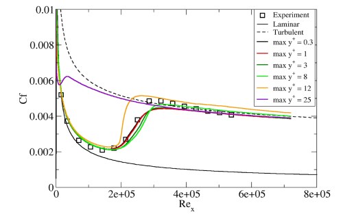
The effect of increasing and decreasing  for a flat plate test case (T3A) is shown in Figure 4.1: Effect of increasing y+ for the flat plate T3A test case and Figure 4.2: Effect of decreasing y+ for the flat plate T3A test case. For
  values between
0.001 and 1, there is almost no effect on the solution. Once the maximum
values between
0.001 and 1, there is almost no effect on the solution. Once the maximum  increases above 8, the transition onset location
begins to move upstream. At a maximum
increases above 8, the transition onset location
begins to move upstream. At a maximum  of 25, the boundary layer is almost completely turbulent.
For
of 25, the boundary layer is almost completely turbulent.
For  values below
0.001, the transition location appears to move downstream. This is
presumably caused by the large surface value of the specific turbulence
frequency
values below
0.001, the transition location appears to move downstream. This is
presumably caused by the large surface value of the specific turbulence
frequency  , which scales with the first grid
point height. Additional simulations on a compressor test case have
indicated that at very small
, which scales with the first grid
point height. Additional simulations on a compressor test case have
indicated that at very small  values the
SST blending functions switch to
values the
SST blending functions switch to  in the boundary
layer. For these reasons, very small (below 0.001)
in the boundary
layer. For these reasons, very small (below 0.001)  values should be avoided at all costs.
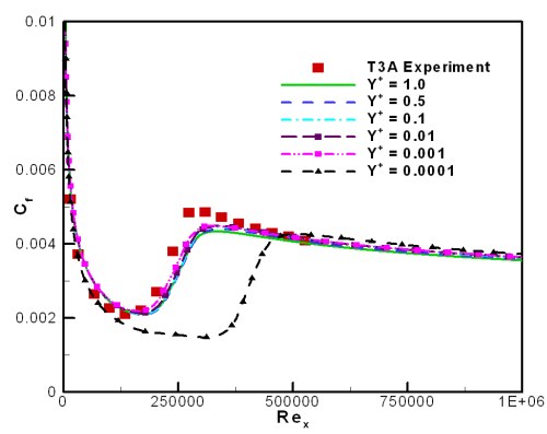
(Figure 4.2: Effect of decreasing y+ for the flat plate T3A test case provided by Likki, Suzen and Huang [102])
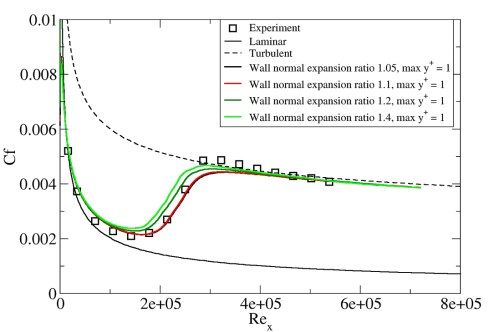
The effect of wall normal expansion ratio from a  value of 1 is shown in Figure 4.3: Effect of wall normal expansion ratio for the flat plate T3A
test case. For expansion factors of 1.05 and 1.1, there
is no effect on the solution. For larger expansion factors of 1.2
and 1.4, there is a small but noticeable upstream shift in the transition
location. Because the sensitivity of the solution to wall-normal grid
resolution can increase for flows with pressure gradients, it is recommended
that you apply grids with
value of 1 is shown in Figure 4.3: Effect of wall normal expansion ratio for the flat plate T3A
test case. For expansion factors of 1.05 and 1.1, there
is no effect on the solution. For larger expansion factors of 1.2
and 1.4, there is a small but noticeable upstream shift in the transition
location. Because the sensitivity of the solution to wall-normal grid
resolution can increase for flows with pressure gradients, it is recommended
that you apply grids with  and
expansion factors smaller than 1.1.
and
expansion factors smaller than 1.1.
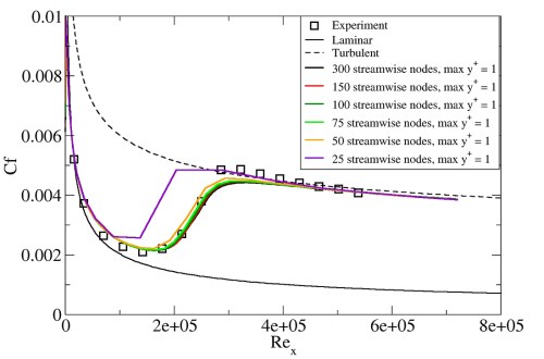
The effect of streamwise grid refinement is shown in Figure 4.5: Effect of streamwise grid density for the flat plate T3A test case. Surprisingly, the model was not very sensitive to the number of streamwise nodes. The solution differed significantly from the grid independent one only for the case of 25 streamwise nodes where there was only one cell in the transitional region. Nevertheless, the grid independent solution appears to occur when there are approximately 75 - 100 streamwise grid points. As well, better streamwise resolution is most likely necessary if separation induced transition takes place. In this case, the number of nodes has to be sufficient to resolve the separation bubble. A general rule is that at least 20 nodes should cover the bubble length. For low Reynolds numbers (<105) the bubble size is comparable to the blade chord length and this requirement is easy to satisfy. Even the recommended 75-100 grid points from the leading to the trailing edge are typically sufficient. However, the bubble decreases as the Reynolds number increases; therefore the grid has to be refined in the regions of the expected separation. An example of how the mesh density influences the resolution of a separation bubble near the leading edge of a wind turbine airfoil is illustrated in Figure 4.4: Effect of streamwise grid density for resolving the separation-induced transition due to a leading edge separation bubble for a wind turbine airfoil. The two meshes shown differ by the number of nodes in streamwise direction in the region covered by the bubble. On Mesh 1, the bubble is resolved by just a few nodes and appears to be much smaller compared to that for the finer mesh, Mesh 2. Clearly, if there are not enough streamwise nodes, the model cannot resolve the rapid separation-induced transition and the boundary layer on the suction side stays laminar, which might have a large influence on the lift coefficient and stall angle predictions.
Note that the high resolution advection scheme has been used for all equations including the turbulent and transition equations and this is the recommended default setting for transitional computations. In CFX, when the transition model is active and the high resolution scheme is selected for the hydrodynamic equations, the default advection scheme for the turbulence and transition equations is automatically set to high resolution.
Figure 4.4: Effect of streamwise grid density for resolving the separation-induced transition due to a leading edge separation bubble for a wind turbine airfoil

One point to note is that for sharp leading edges, often transition can occur due to a small leading edge separation bubble. If the grid is too coarse, the rapid transition caused by the separation bubble is not captured.
Based on the grid sensitivity study the recommended best practice
mesh guidelines are a max  of 1, a wall
normal expansion ratio of 1.1 and about 75 - 100 grid nodes in the
streamwise direction. Note that if separation induced transition is
present, additional grid points in the streamwise direction are most
likely needed. For a typical 2D blade assuming an H-O-H type grid,
the above guide lines result in an inlet H-grid of 15x30, an O-grid
around the blade of 200x80 and an outlet H-grid of 100x140 for a total
of approximately 30 000 nodes, which has been found to be grid independent
for most turbomachinery cases. It should also be noted that for the
surfaces in the out of plane z-direction, symmetry planes should always
be used, not slip walls. The use of slip walls has been found to result
in an incorrect calculation of the wall distance, which is critical
for calculating the transition onset location accurately. Another
point to note is that all the validation cases for the transition
model have been performed on hexahedral meshes. At this point, the
accuracy of the transition model on tetrahedral meshes has not been
investigated.
of 1, a wall
normal expansion ratio of 1.1 and about 75 - 100 grid nodes in the
streamwise direction. Note that if separation induced transition is
present, additional grid points in the streamwise direction are most
likely needed. For a typical 2D blade assuming an H-O-H type grid,
the above guide lines result in an inlet H-grid of 15x30, an O-grid
around the blade of 200x80 and an outlet H-grid of 100x140 for a total
of approximately 30 000 nodes, which has been found to be grid independent
for most turbomachinery cases. It should also be noted that for the
surfaces in the out of plane z-direction, symmetry planes should always
be used, not slip walls. The use of slip walls has been found to result
in an incorrect calculation of the wall distance, which is critical
for calculating the transition onset location accurately. Another
point to note is that all the validation cases for the transition
model have been performed on hexahedral meshes. At this point, the
accuracy of the transition model on tetrahedral meshes has not been
investigated.
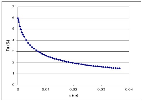
It has been observed that the turbulence intensity specified
at an inlet can decay quite rapidly depending on the inlet viscosity
ratio  (and hence turbulence
eddy frequency). As a result, the local turbulence intensity downstream
of the inlet can be much smaller than the inlet value (see Figure 4.6: Decay of turbulence intensity (Tu) as a function of streamwise
distance (x)). Typically, the larger the
inlet viscosity ratio, the smaller the turbulent decay rate. However,
if too large a viscosity ratio is specified (that is, >100), the skin
friction can deviate significantly from the laminar value. There is
experimental evidence that suggests that this effect occurs physically;
however, at this point it is not clear how accurately the transition
model reproduces this behavior. For this reason, if possible, it is
desirable to have a relatively low (that is
(and hence turbulence
eddy frequency). As a result, the local turbulence intensity downstream
of the inlet can be much smaller than the inlet value (see Figure 4.6: Decay of turbulence intensity (Tu) as a function of streamwise
distance (x)). Typically, the larger the
inlet viscosity ratio, the smaller the turbulent decay rate. However,
if too large a viscosity ratio is specified (that is, >100), the skin
friction can deviate significantly from the laminar value. There is
experimental evidence that suggests that this effect occurs physically;
however, at this point it is not clear how accurately the transition
model reproduces this behavior. For this reason, if possible, it is
desirable to have a relatively low (that is  1 - 10) inlet
viscosity ratio and to estimate the inlet value of turbulence intensity
such that at the leading edge of the blade/airfoil, the turbulence
intensity has decayed to the desired value.
1 - 10) inlet
viscosity ratio and to estimate the inlet value of turbulence intensity
such that at the leading edge of the blade/airfoil, the turbulence
intensity has decayed to the desired value.
The decay of turbulent kinetic energy can be calculated with the following analytical solution:
 | (4–3) |
For the SST turbulence model in the freestream the constants are:
 | (4–4) |
The time scale can be determined as follows:
 | (4–5) |
where  is the streamwise distance downstream
of the inlet and
is the streamwise distance downstream
of the inlet and  is the mean convective velocity.
The eddy viscosity is defined as:
is the mean convective velocity.
The eddy viscosity is defined as:
 | (4–6) |
The decay of turbulent kinetic energy equation can be rewritten
in terms of inlet turbulence intensity ( ) and eddy viscosity ratio (
 ) as follows:
 | (4–7) |
You should ensure that the  values
around the body of interest roughly satisfy
values
around the body of interest roughly satisfy  . For smaller values of
  , the
reaction of the SST model production terms to the transition onset
becomes too slow and transition can be delayed past the physically
correct location.
, the
reaction of the SST model production terms to the transition onset
becomes too slow and transition can be delayed past the physically
correct location.
Simulations of external aerodynamic flows typically require
a computational domain with remote outer boundaries. In such cases,
it might be necessary to specify excessively high values of turbulence
intensity and eddy viscosity ratio at the inlet in order to get the
desired value at the airfoil. In addition, numerical grids around
aerodynamic bodies typically feature very coarse grids at the far-field
boundary. For such coarse grids, Equation 4–7 is no longer accurately resolved and the numerical decay can differ
substantially from the analytical one. Alternatively, sensible inlet
values can be obtained if the onset of the  decay
is shifted closer to the airfoil. This can be implemented via adding
source terms into the
decay
is shifted closer to the airfoil. This can be implemented via adding
source terms into the  and
and  equations, which keep the inlet values
of the transported variables unchanged until the specified coordinate.
These source terms read as:
equations, which keep the inlet values
of the transported variables unchanged until the specified coordinate.
These source terms read as:


where  is an arbitrary coordinate between the computational domain inlet
and the airfoil. The two source terms are actually the inverted sign
sink terms for the SST model when it is working in the
is an arbitrary coordinate between the computational domain inlet
and the airfoil. The two source terms are actually the inverted sign
sink terms for the SST model when it is working in the  regime. Adding these terms prevents
  and
and  values from undergoing any
decay in the freestream until the
values from undergoing any
decay in the freestream until the  location
is reached. The streamwise distance in Figure 4.6: Decay of turbulence intensity (Tu) as a function of streamwise
distance (x) counts
then from the
location
is reached. The streamwise distance in Figure 4.6: Decay of turbulence intensity (Tu) as a function of streamwise
distance (x) counts
then from the  coordinate. More
general
coordinate. More
general  functions can be used, but it needs to be ensured
that
functions can be used, but it needs to be ensured
that  is zero in the vicinity of the wall boundary layers
around the aerodynamic body.
is zero in the vicinity of the wall boundary layers
around the aerodynamic body.
Proper grid refinement and specification of inlet turbulence levels is crucial for accurate transition prediction. In general, there is some additional effort required during the grid generation phase because a low-Re grid with sufficient streamwise resolution is needed to accurately resolve the transition region. As well, in regions where laminar separation occurs, additional grid refinement is necessary in order to properly capture the rapid transition due to the separation bubble. Finally, the decay of turbulence from the inlet to the leading edge of the device should always be estimated before running a solution as this can have a large effect on the predicted transition location.