


CFX has the capability to model fluid mixtures consisting of an arbitrary number of separate physical components (or "species"). Each component fluid may have a distinct set of physical properties. The CFX-Solver will calculate appropriate average values of the properties for each control volume in the flow domain, for use in calculating the fluid flow. These average values will depend both on component property values and on the proportion of each component present in the control volume.
This section describes how to model multicomponent flow simulations, in addition to offering modeling advice.
In multicomponent flow, assume that the various components of a fluid are mixed at the molecular level, that they share the same mean velocity, pressure and temperature fields, and that mass transfer takes place by convection and diffusion. The more complex situation involving fluid interfaces, where different components are mixed on larger scales and may have separate velocity and temperature fields is called multiphase flow. This type of flow cannot be modeled with the multicomponent model. For details, see Multiphase Flow Modeling.
It is further assumed that the diffusion velocity of a component obeys Fick’s Law.
The following terms are used in CFX multicomponent flow. Examples to illustrate the difference between fluids and components are shown in the next section. For details, see Multicomponent Flow Examples.
A pure substance is a material with specified physical properties, such as density and viscosity. These properties may be numeric constants, or the CFX Expression Language (CEL) may be used to specify non-constant properties.
A component is one part of a multicomponent fluid. When a pure substance is used as part of a multicomponent fluid it is referred to as a component of that fluid. A fixed composition mixture could also be treated as a component of another fluid. The properties of a component are calculated from the mass fractions of the constituent materials and are based on the materials forming an ideal mixture below. For details, see Ideal Mixture.
A multicomponent fluid contains two or more components and its properties are calculated from those of the constituent components. The components are assumed to be mixed at the molecular level and the properties of the fluid are dependent on the proportion of its components.
The components can exist in fixed mass fractions (Fixed Composition Mixture) or in variable mass fractions (Variable Composition Mixture). For Variable Composition Mixtures, the proportions of each component present may vary in space or time. This may be caused by the conversion of one component to another through a chemical reaction, such as combustion, driven by diffusion or caused by specifying different proportions at different boundaries or in the initial conditions.
In the solution to a multicomponent simulation, a single velocity field is calculated for each multicomponent fluid and written to the results file. Individual components move at the velocity of the fluid of which they are part, with a drift velocity superimposed, arising from diffusion.
The properties of multicomponent fluids are calculated on the assumption that the constituent components form an ideal mixture below. For details, see Ideal Mixture.
Additional Variables are non-reacting, scalar components that are transported through the flow. Additional Variables can be used to model the transport of a passive material in the fluid flow, such as smoke in air and dye in water, or to model other scalar variables, such as electric field. The presence of an Additional Variable does not affect the fluid flow by default, although some fluid properties may be defined to depend upon an Additional Variable by means of the CFX Expression Language. Additional Variables may be carried by, as well as diffuse through, the fluid; they are typically specified as concentrations.
An ideal mixture is a mixture of components such that the properties of the mixture can be calculated directly from the properties of the components and their proportions in the mixture.
If the flow of a component is modeled using a transport equation, then it is transported with the fluid and may diffuse through the fluid, and its mass fraction is calculated accordingly.
If the flow of a component is modeled using a constraint equation, its mass fraction is calculated to ensure that all the component mass fractions sum to unity, that is, the mass fraction of the component is set equal to the total mass fractions of the other components in the same fluid subtracted from unity.
All pure substances and multicomponent fluids are specified in the Materials details view. This can be accessed from the Materials workspace in CFX-Pre. A description of the use of the Materials details view is available in Material Details View: Pure Substance in the CFX-Pre User's Guide. In this section, the relation between fluids and components is discussed.
The following example shows a CFD simulation of a tank that
contains two fluids, Water and Atmosphere. Water is a pure substance (single-component
fluid) while Atmosphere is a Variable
Composition Mixture containing Air and Pollutant. Pollutant is a Pure Substance while Air is a Fixed Composition Mixture made from other
pure substances.
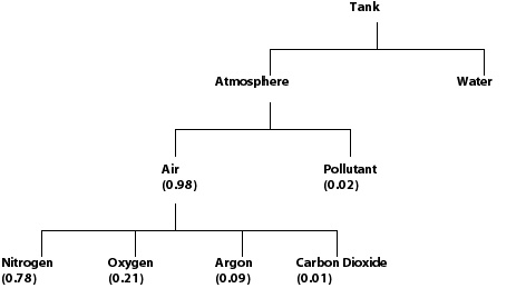
You cannot nest Fixed and Variable Composition Mixtures further than as shown in this example (for example, Fixed Composition Mixtures cannot be made from other Fixed Composition Mixtures).
Because there is more than one fluid, this is a multiphase simulation (regardless of whether or not the fluids have the same phase). For details, see Multiphase Flow Modeling.
This example illustrates the relationship between components, fluids, and Additional Variables.
Smoke in Air can be considered in a number
of different ways:
The flow can be considered to be that of a single fluid,
Air. The smoke is modeled as an Additional Variable using a transport equation. For details, see:Using this model, it is assumed that the presence of the smoke does not affect the air flow. It is, therefore, most suitable for small concentrations of small smoke particles.
The flow can be considered to be a multicomponent fluid, consisting of two components:
SmokeandAir. Using this model, the presence ofSmokewill affect the flow of the fluid through the fluid properties. However, the smoke and air are assumed to have a common velocity. This model could be used for larger concentrations of small smoke particles.The flow can be considered to be that of a single fluid,
Air, with the smoke particles modeled using particle tracking.
Component mass fractions can be calculated by the CFX-Solver using a Transport Equation, an Algebraic Equation and the Constraint condition. Additionally, they can be based on a flamelet library or they can use the algebraic slip model. For details, see:
If an Algebraic Equation is used, you should enter a CEL expression that evaluates to values between 0 and 1 throughout the domain. This describes the mass fraction of the component. When more than one component uses an Algebraic Equation, the sum of the mass fractions at any location must be less than or equal to 1.
If the Transport Equation option is used, CFX solves for the transport and diffusion of the component. At least one component must be solved for using a transport equation.
The mass fractions of the components must always add up to 1. This is enforced by specifying one component as the constrained component. The mass fraction of this component is always the difference between 1 and the sum of the mass fractions of all other components. Exactly one component must use Constraint as the option. This results in the following restrictions:
When only two components exist, one component must use the Transport Equation option and one must use the Constraint option.
When more than two components exist, one component must use the Transport Equation option, one must use the Constraint option and the remaining components can use either the Transport Equation option or the Algebraic Equation option.
An Automatic option is also available; this will set the option to either Transport Equation or Library. If the combustion model is:
NoneEddy DissipationFinite Rate ChemistryFinite Rate Chemistry and Eddy Dissipation
then Automatic will translate into Transport Equation. If the combustion model is:
Laminar Flamelet with PDFPartially Premixed and Laminar Flamelet with PDF
then Automatic will translate into Library. For details, see Flamelet Libraries in the CFX-Solver Theory Guide.
The Automatic option will not set any component as the Constraint component, so you must change at least one component from Automatic to Constraint in CFX-Pre.
The Algebraic Slip model is a multiphase model. For details, see Algebraic Slip Model (ASM).
If a Transport Equation is being solved, you can enter a value for the Kinematic Diffusivity. If a value is not set, then either the dynamic viscosity (unity Schmidt number assumption for cases without heat transfer) or the thermal conductivity (unity Lewis number assumption for cases with heat transfer) of the fluid is used to derive the molecular diffusion coefficient for all components (see Multicomponent Energy Diffusion for further information).
Turbulent diffusivity is not affected by this setting. A fluid property is a weighted average of the component properties based on the local mass fractions. If you would like to set the dynamic diffusivity, simply set the kinematic diffusivity as an expression equal to the intended value of the dynamic diffusivity divided by the density.
If the component model is set to either transport equation or to Algebraic Slip, then you may optionally enable the specification of the Turbulent Flux Closure. When the specification is not enabled, the default is to apply the same settings as for the energy equation, see Heat Transfer.
The Turbulent Flux Closure option can be used for specification of component-dependent turbulent Schmidt numbers, which may be non-constant using expressions (CEL).
The implementation of boundary conditions for multicomponent flow is very similar to that for single-component flow.
(Physical description)
Boundary Conditions in the CFX-Solver Theory Guide
(Mathematical models)
However, you need to specify mass fractions of components on inlet and opening type boundary conditions.
This option is used to control the numerical treatment for the energy diffusion term for multicomponent fluids. There are two modes: The generic formulation and the unity Lewis number formulation, which are valid only under certain conditions. For details, see Multicomponent Energy Diffusion in the CFX-Solver Theory Guide. The less general mode can significantly reduce the numerical cost for assembly of the energy equation, in particular when the fluid has a large number of components.
Three options are available:
Automaticforces the solver to use the numerically efficient unity Lewis number assembly when physically valid, and use the generic assembly otherwise; this is the default.
Generic Assemblyforces the solver to use the general enthalpy diffusion term; the default molecular diffusivity for mass fractions is equal to the fluid viscosity (unity Schmidt number,
 =
1). Use this option to revert to the behavior of CFX release 5.7.1
or previous.
=
1). Use this option to revert to the behavior of CFX release 5.7.1
or previous.Unity Lewis Numberforces the solver to use the unity Lewis number formulation; the default molecular diffusivity for mass fractions is thermal conductivity divided by heat capacity (unity Lewis number,
 =
1).
=
1).Generic Molecular and Unity Turbulentforces the solver to use the general formulation for molecular transport and the unity Lewis number formulation for turbulent transport; the default molecular diffusivity for mass fractions is equal to the fluid viscosity (unity Schmidt number,
 = 1). Use this option to revert to the behavior of CFX release
5.7.1 or previous.
= 1). Use this option to revert to the behavior of CFX release
5.7.1 or previous.Unity Molecular and Generic Turbulentforces the solver to use the unity Lewis number formulation for molecular transport and the general formulation for turbulent transport; the default molecular diffusivity for mass fractions is thermal conductivity divided by heat capacity (unity Lewis number,
 = 1).
= 1).
Note: Forcing Unity Lewis Number mode when
not appropriate may lead to inconsistent energy transport. For example,
this option should not be used in combination with user-specified
component diffusivities. Therefore, using the Unity Lewis
Number option is not recommended.
For multicomponent fluids, the effective assembly options for molecular and turbulent energy transport, respectively, are reported to the CFX-Solver Output file in the section Multi-Component Specific Enthalpy Diffusion. For details, see Multicomponent Specific Enthalpy Diffusion (MCF) in the CFX-Solver Manager User's Guide.
For single-component fluids or for isothermal flow the option has no effect. In the latter case the fluid viscosity is applied as the default molecular diffusivity for components.