The Detached Eddy Simulation is a combination of RANS and LES methods. In an alternative approach, a new class of URANS models has been developed that can provide a LES-like behavior in detached flow regions (Menter et al. [132], Menter and Egorov [130], Menter and Egorov [131], Egorov and Menter [197]). The Scale-Adaptive Simulation (SAS) concept is based on the introduction of the von Karman length-scale into the turbulence scale equation. The information provided by the von Karman length-scale allows SAS models to dynamically adjust to resolved structures in a URANS simulation, which results in a LES-like behavior in unsteady regions of the flowfield. At the same time, the model provides standard RANS capabilities in stable flow regions.

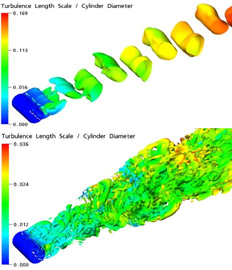
Figure 4.10: Resolved structures for cylinder in cross flow (top: URANS; bottom: SAS-SST) shows isosurfaces where for a cylinder in cross flow (Re=3.6x10⁶), calculated using the SST model (URANS) and the SAS-SST model. The URANS simulation produces only the large-scale unsteadyness, whereas the SAS-SST model adjusts to the already resolved scales in a dynamic way and allows the development of a turbulent spectrum in the detached regions.

Figure 4.10: Resolved structures for cylinder in cross flow (top: URANS; bottom: SAS-SST)

The original version of the SST-SAS model (Menter and Egorov [131]) has undergone continued evolution. This model is still available in Ansys CFX, but the latest version of the SAS model (Egorov and Menter [197]) is now the default model. More details can be found in Scale-Adaptive Simulation Theory in the CFX-Solver Theory Guide.

The SAS method is an improved URANS formulation, with the ability to adapt the length scale to resolved turbulent structures. In order for the SAS method to produce a resolved turbulent spectrum, the underlying turbulence model has to go unsteady. This is typically the case for flows with a global instability, as observed for flows with large separation zones, or vortex interactions. There are many technical flows, where steady-state solutions cannot be obtained or where the use of smaller timesteps results in unsteady solutions. One could argue that the occurrence of unsteady regions in a RANS simulation is the result of a non-local interaction, which cannot be covered by the single-point RANS closure. All these flows will benefit from the SAS methodology.

On the other hand, there are classes of flows where the SAS model will return a steady solution. The two main classes are attached or mildly separated boundary layers and undisturbed channel/pipe flows. These flows (or areas in a complex flow domains) will be covered by the RANS formulation. This behavior of SAS is ideal for many technical applications, as flows for which the model produces steady solutions are typically those, where a well-calibrated RANS model can produce accurate results.

Contrary to DES, SAS cannot be forced to go unsteady by grid refinement. However, it has been shown in the backstep simulation above that enforcing unsteadiness by grid refinement does require an in-depth understanding of the flow, the turbulence model and its interaction with the grid to produce reliable results. Nevertheless, there will be cases where the grid sensitivity of DES will be advantageous, as it allows unsteady simulations where SAS might produce a steady-state flow-field.

This leads to the following hierarchy of models of increased complexity, which can be used as a guideline in order to estimate the needed effort: