


This tutorial demonstrates the turbomachinery postprocessing capabilities of CFD-Post.
In this example, you will read Fluent case and data files (without doing any calculations) and perform a number of turbomachinery-specific postprocessing operations.
This tutorial demonstrates:
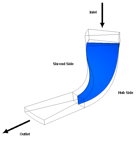
This tutorial considers the problem of a centrifugal compressor shown schematically in Figure 3.1: Problem Specification. The model is composed of a single 3D sector of the compressor to take advantage of the circumferential periodicity in the problem. The flow of air through the compressor is simulated and the postprocessing capabilities of CFD-Post are used to display realistic, full 360° images of the solution obtained.
If this is the first tutorial you are working with, it is important to review Introduction to the Tutorials before beginning.
Create a working directory.
CFD-Post uses a working directory as the default location for loading and saving files for a particular session or project.
Download the
turbo.zipfile here .Unzip
turbo.zipto your working directory.Ensure that the following tutorial input files are in your working directory:
turbo.cas.gz
turbo.cdat.gz
Before you start CFD-Post, set the working directory. The procedure for setting the working directory and starting CFD-Post depends on whether you run CFD-Post stand-alone, from the Ansys CFX Launcher, or from Ansys Workbench:
To run CFD-Post stand-alone
On Windows:
From the Start menu, right-click All Programs > ANSYS 2024 R2 > Fluid Dynamics > CFD-Post 2024 R2 and select Properties.
Type the path to your working directory in the Start in field and click .
Click All Programs > ANSYS 2024 R2 > Fluid Dynamics > CFD-Post 2024 R2 to launch CFD-Post.
On Linux, enter
cfdpostin a terminal window that has its path set up to run CFD-Post. The path will be something similar to/usr/ansys_inc/v242/CFD-Post/bin.
To run Ansys CFX Launcher
Start the launcher.
You can run the launcher in any of the following ways:
On Windows:
From the Start menu, select All Programs > ANSYS 2024 R2 > Fluid Dynamics > CFX 2024 R2.
In a Command Prompt that has its path set up correctly to run CFX, enter
cfx5launch. If the path is not set up correctly, you will need to type the full pathname of thecfxcommand, which will be something similar toC:\Program Files\ANSYS Inc\v242\CFX\bin.
On Linux, enter
cfx5launchin a terminal window that has its path set up to run CFX. The path will be something similar to/usr/ansys_inc/v242/CFX/bin.
Set the working directory.
Click the CFD-Post 2024 R2 button.
Ansys Workbench
Start Ansys Workbench.
From the menu bar, select File > Save As and save the project file to the directory that you want to be the working directory.
Open the Component Systems toolbox and double-click Results. A Results system opens in the Project Schematic.
Right-click the A2 Results cell and select Edit. CFD-Post opens.
In the steps that follow, you will explore the solution using CFD-Post.
- 3.4.1. Prepare the Case and Set the Viewer Options
- 3.4.2. Initialize the Turbomachinery Components
- 3.4.3. Compare the Blade-to-Blade, Meridional, and 3D Views
- 3.4.4. Display Pressure on Meridional Isosurfaces
- 3.4.5. Display a 360-Degree View
- 3.4.6. Calculate and Display Values of Variables
- 3.4.7. Display the Inlet to Outlet Chart
- 3.4.8. Generate and View a Turbo Report
Load the CDAT file (turbo.cdat.gz) from the menu bar by selecting File > Load Results. In the Load Results File dialog box, select turbo.cdat.gz and click .
If you see a message that discusses Global Variables Ranges, it can be ignored. Click .
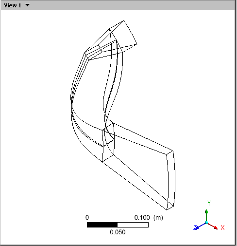
The turbo blade appears in the viewer in an isometric orientation. The Wireframe appears in the 3D Viewer and there is a check mark beside Wireframe in the Outline workspace; the check mark indicates that the wireframe is visible in the 3D Viewer.
Set CFD-Post to display the units you want to see. These display units are not necessarily the same types as the units in the results files you load; however, for this tutorial you will set the display units to be the same as the solution units.
Right-click the viewer and select Viewer Options.
In the Options dialog box, select Common > Units.
Set System to SI and click .
Note: The display units you set are saved between sessions and projects. This means that you can load results files from diverse sources and always see familiar units displayed.
Double-click Wireframe in the Outline workspace to see the details view. To display the mesh, set Edge Angle to 0 degrees and click . The edge angle determines how much of the surface mesh is visible. If the angle between two adjacent faces is greater than the edge angle, then that edge is drawn. If the edge angle is set to 0°, the entire surface mesh is drawn. If the edge angle is large, then only the most significant corner edges of the geometry are drawn.
Tip: With the mouse focus on CFD-Post and the mouse over the Details of Wireframe editor, press F1 to see help about the Wireframe object.
On the Wireframe details view, click and to restore the original settings.
Optionally, set the viewer background to white:
Right-click the viewer and select Viewer Options.
In the Options dialog box, select CFD-Post > Viewer.
Set:
Background > Color Type to Solid.
Background > Color to white. To do this, click the bar beside the Color label to cycle through 10 basic colors. (Click the right-mouse button to cycle backwards.) Alternatively, you can choose any color by clicking
 icon to the right of the Color option.
 Text Color to black (as above).
Edge Color to black (as above).
Click to have the settings take effect.
Before you can start using the Turbo workspace features, you need to initialize the components of the loaded case (such as hub, blade, periodics, and so on). Among other things, initialization generates span, a (axial), r (radial), and Theta coordinates for each component.
You need to initialize Fluent case and data files manually (automatic initialization is available only for CFX files produced by the Turbo wizard in CFX-Pre). To initialize the components:
Click the Turbo tab in the upper-left pane of the CFD-Post window. The Turbo workspace appears as does a Turbo initialization dialog box that offers to auto-initialize all turbo components. Click .
In the Turbo workspace under Initialization, double-click
fluid (fluid). The details view of Fluid appears.On the Definition tab, the regions of the geometry are listed under Turbo Regions. However, not all regions are listed; correct this as follows:
Click Location editor
to the right of the Hub region.Hold down the Ctrl key and in the Location Selector select
wall diffuser hub,wall hub, andwall inlet hub.Click .
The Hub field now lists all three hub locations.
Repeat the previous steps for the Shroud region, selecting
wall diffuser shroud,wall inlet shroud, andwall shroud.Repeat the previous steps for the Blade region, selecting only
wall blade.Repeat the previous steps for the Inlet region, selecting only
inlet.Repeat the previous steps for the Outlet region, selecting only
outlet.Repeat the steps for the Periodic 1 region, selecting
periodic.33,periodic.34, andperiodic.35.You do not need to initialize the
periodic.*shadowregions; theperiodic.*nodes provide the information that the turbo reports require.
Click the Instancing tab.
Ensure that Number of Graphical Instances is set to
1.Ensure that Axis Definition is set to
Custom, that Method is set toPrincipal Axis, and that Axis is set toZ.Set Instance Definition to
Custom.Select Full Circle.
Click . This generates variables that you will use later to create reports.
Tip: If the turbo topology is not correctly defined, an error message is generated and the initialization does not occur. To resolve such an error:
Ensure that the rotational axis is correct.
Ensure that the turbo regions are correctly set, and that they enclose the passage without any gaps.
Double-click at the top of the Turbo tree view. The Initialization editor appears.
Click the Calculate Velocity Components button. This generates velocity variables that you will also use in your reports.
The initialization process has created a variety of plots automatically; you will access these from the Turbo tab in the sections that follow.
To compare the Blade-to-Blade, Meridional, and 3D Views:
In the Turbo workspace, select the Three Views option at the bottom of the Initialization editor. In the 3D Viewer you can see the Turbo Initialization View, the Blade to Blade View, and the Meridional View.
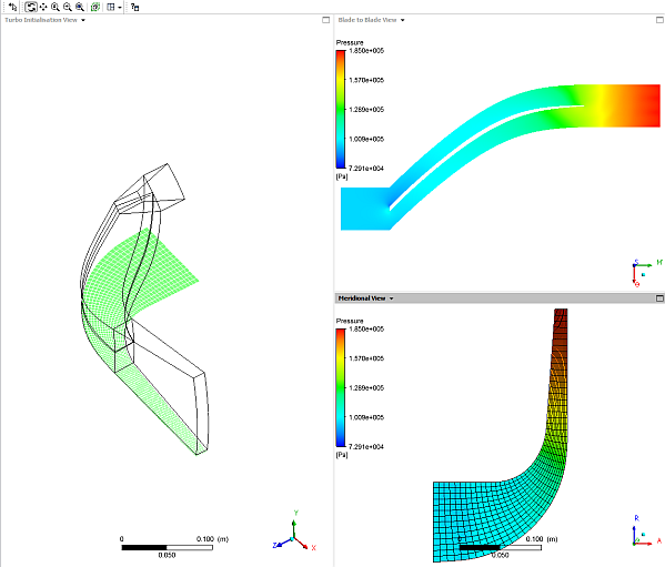
The CFD-Post Blade to Blade View is equivalent
to the Fluent "2D contour on a spanwise surface". By
default, the variable shown is Pressure.
To change this to velocity and to make the image more like the default Fluent equivalent:
In the Blade to Blade View, right-click the colored area shown in the viewport and select Edit.
In the details view for the Blade-to-Blade Plot, change the Plot Type from
ColortoContour(this changes the continuous gradation found inColorto the discrete color bands found inContour).Change Variable to
Velocity.Change the # of Contours to
21.Click .
The CFD-Post Meridional View is equivalent to the Fluent "contour averaged in the circumferential direction". To make the image more like the default Fluent equivalent:
In the Meridional View, right-click the colored area shown in the viewport and select Edit.
In the details view for the Meridional Plot, change the Plot Type from
ColortoContour.Change the # of Contours to
21.Click .
In this example you will define six meridional isosurfaces colored by pressure.
Return to the original orientation of the case:
In the Tree view, double-click Plots and select Single View.
Double-click 3D View.
From the menu bar select Insert > Location > Isosurface and accept the default name.
Set the following values on the details view for the isosurface:
Tab
Field
Value
Geometry
Domains
fluid
Variable
Linear BA Streamwise Location
[a]Value
.01
Color
Mode
Variable
Variable
Pressure
Range
User Specified
Min
72800 [Pa]
Max
186000 [Pa]
Render
Lighting
(Cleared)
Click to define the isosurface.
Right-click Isosurface 1 in the Tree view and select Duplicate, then change Geometry > Value to
.2and click .Create other duplicates for geometry values
.4,.6,.8, and.99.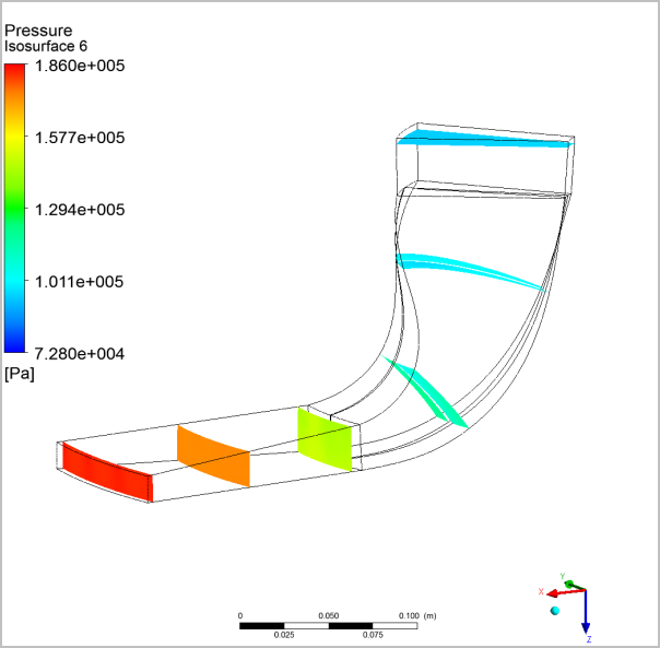
Note: You can set locator variables other than Linear BA (Blade Aligned) Streamwise Location. For example, edit Isosurface 5 and change
Linear BA Streamwise LocationtoM Length Normalizedto see how the isosurface changes.
To display a 360° view of the turbomachinery:
In the Outline tree view, right-click any object under
User Locations and Plotsthat has a visibility check box, then select Hide All.Under User Locations and Plots, ensure that the check box beside
Wireframeis selected.Under Cases > turbo, double-click fluid to edit that domain.
On the Instancing tab:
Set Number of Graphical Instances to
20.Ensure that Instance Definition is set to
Customand that Full Circle is selected.Ensure that Axis Definition is set to
Custom, that Method is set toPrincipal Axis, and that Axis is set toZ.
Click .
If necessary, click the Fit View
 icon so that you can see the whole case.
You can calculate the values of variables at locations in the case and display these results in a table. First, use the Function Calculator to see how to create a function.
From the menu bar, select Tools > Function Calculator. The Calculators tab appears with the Function Calculator displayed.
Use the Function Calculator to calculate the mass flow average of pressure at the inlet as follow:
Use the Function drop-down arrow to select
massFlowAve.Use the Location drop-down arrow to select
inlet.Use the Variable drop-down arrow to select
Pressure.At the bottom of the Function Calculator select Show equivalent expression.
Click and the expression and results appear:
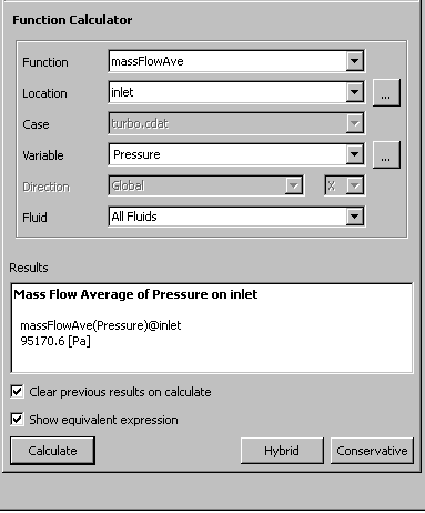
The Function Calculator not only makes it easy to create and calculate a function, it also enables you to see the syntax for functions, which you will use in the subsequent steps.
To display functions like this in a table, click the Table Viewer tab (at the bottom of the viewer area). The Table Viewer appears.
In the toolbar at the top of the Table Viewer, click New Table
 . The New Table dialog box appears. Type in
 Inlet and Outlet Valuesand click .Type the following text to make cell headings:
In cell B1: Inlet
In cell C1: Outlet
In cell A2: Mass Flow
In cell A3: Average Pressure
Now, create functions:
Click in cell B2, then in the Table Viewer toolbar, select Function > CFD-Post > massFlow. The definition
=massFlow()@appears.With the text cursor after the @ symbol, click Location > inlet.
Press Enter; the value of the mass flow at the inlet appears.
Repeat the above steps for cell C2, but use Location > outlet.
For cell B3, select Function > CFD-Post > massFlowAve. With the text cursor between the parentheses, select Variable > Pressure. With the text cursor after the @ symbol, click Location > inlet. Press Enter; the value of the mass flow average of pressure at the inlet appears.
Repeat the previous step for cell C3, but use Location > outlet.
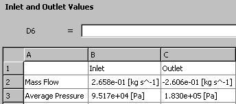
Your table should be similar to this:
Format the cells to make the table easier to read.
Click in cell A1 and, while holding down Shift, click in cell C1. Now the operations you perform will apply to A1 through C1.
Click
 to make the heading font bold,
then click
to make the heading font bold,
then click  to center the heading text. Click
  to apply a background color to those cells.
Click in cell A2 and, while holding down Shift, click in cell A3. Click
to make the row description bold,
then click  to right-align the text.
Manually resize the cells.
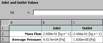
Your table should be similar to this:
Click the Report Viewer tab and then click in the Report Viewer toolbar. The table data appears at the bottom of the report.
In CFD-Post, displaying the Inlet to Outlet chart is equivalent to displaying averaged XY plots in Fluent. To display the Inlet to Outlet chart:
In the Turbo workspace's Turbo Charts area, double-click Inlet to Outlet.
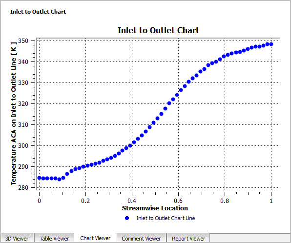
Now, change the chart to compare temperature to streamwise location (the latter being called "meridional location" in Fluent) and make the chart look more like the Fluent default:
Set the following:
Setting
Value
Domains
fluid
Samples/Comp
60
Y Axis
> Variable
Temperature
Click Apply. The chart appears:
Click the Report Viewer tab at the bottom of the viewer area.
In the Report Viewer toolbar, click the button. The Inlet to Outlet Chart appears in the User Data section of the report.
Tip: You can also explore the other Turbo Charts:
Blade Loading
Circumferential
Hub to Shroud
Turbo reports give performance results, component data summary tables, meanline 1D charts, stage plots, and spanwise loading charts for the blade.
Note: The Turbo report is generated from the values set when you initialized the case, so if there were any changes required to those values, you would make them now and run the initialization procedure again. For this tutorial, that will not be necessary.
To generate a Turbo report:
Create a new variable that the report expects (which would be available with CFX results files for rotating machinery applications, but which is not available from Fluent case and data files).
From the toolbar, click Variable
 . The Insert Variable dialog
box appears.
. The Insert Variable dialog
box appears.In the Name field, type
Rotation Velocityand click .The details view for Rotation Velocity appears.
In the Expression field, type
Radius * abs(omega) / 1 [rad]and click . This expression calculates the angular speed (in units of length per unit time) as a product of the local radius and the rotational speed.
In the 3D Viewer toolbar, click Fit View
. This ensures that the graphics will not be truncated
in the report you are about to generate.In the Outline tree view, right-click Report and select Report Templates. The Report Templates dialog box appears.
Select an appropriate report template; in this case, select
Centrifugal Compressor Report.Click . The Report Templates dialog box disappears and you can watch the report's progress in the status bar in the bottom-right corner of CFD-Post.
Note: A dialog box appears that warns that hybrid values do not exist and that conservative values will be used. This is expected behavior when using data loaded from Fluent. An error about "Mach Number in Stn Frame" is also mentioned; this prevents a line in the report from appearing. Click .
When the report has been generated, there are new entries in the Outline tree view under Report.
Under User Locations and Plots, double-click
fluid Instance Transform. This is an instance transform generated by the report to facilitate showing two blades in the figures that show blade-to-blade views.Ensure that Number of Passages is set to
20and click .Click the Expressions tab. Double-click the expression fluid Components in 360 to edit it. Change the definition to
20and click .
To view the Turbo report:
In the Report Viewer, click Refresh. The turbo report appears.
Optionally, you can remove pieces from the report by clearing the appropriate check boxes in the Report section of the Outline tree. When you have made your selections, return to the Report Viewer and click Refresh (in the Report Viewer toolbar). The edited version of the turbo report appears.
To produce an HTML version of the report that you can share with others, click Publish (at the top of the viewer area). The report is saved in a filename of your choosing in your working directory (by default).