


This tutorial illustrates how to use CFD-Post to visualize a three-dimensional turbulent fluid flow and heat transfer problem in a mixing elbow. The mixing elbow configuration is encountered in piping systems in power plants and process industries. It is often important to predict the flow field and temperature field in the area of the mixing region in order to properly design the junction.
This tutorial demonstrates how to do the following:
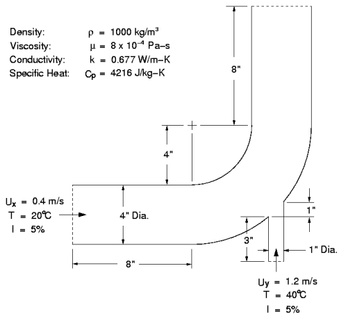
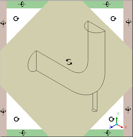
The problem to be considered is shown schematically in Figure 2.1: Problem Specification. A cold fluid at 20° C flows into the pipe through a large inlet and mixes with a warmer fluid at 40° C that enters through a smaller inlet located at the elbow. The pipe dimensions are in inches, but the fluid properties and boundary conditions are given in SI units. The Reynolds number for the flow at the larger inlet is 50,800, so the flow has been modeled as being turbulent.
Note: This tutorial is derived from an existing Fluent case. The combination of SI and Imperial units is not typical, but follows a Fluent example.
Because the geometry of the mixing elbow is symmetric, only half of the elbow is modeled.
If this is the first tutorial you are working with, it is important to review Introduction to the Tutorials before beginning.
Create a working directory.
CFD-Post uses a working directory as the default location for loading and saving files for a particular session or project.
Download the
mixing_elbow.zipfile here .Unzip
mixing_elbow.zipto your working directory.Ensure that the following tutorial input files are in your working directory:
elbow_tracks.xml
elbow1.cas.gz
elbow1.cdat.gz
elbow3.cas.gz
elbow3.cdat.gz
Before you start CFD-Post, set the working directory. The procedure for setting the working directory and starting CFD-Post depends on whether you launch CFD-Post stand-alone, from the Ansys CFX Launcher, or from Ansys Workbench:
To run CFD-Post stand-alone
On Windows:
From the Start menu, right-click All Programs > ANSYS 2024 R2 > Fluid Dynamics > CFD-Post 2024 R2 and select Properties.
Type the path to your working directory in the Start in field and click .
Click All Programs > ANSYS 2024 R2 > Fluid Dynamics > CFD-Post 2024 R2 to launch CFD-Post.
On Linux, enter
cfdpostin a terminal window that has its path set up to run CFD-Post. The path will be something similar to/usr/ansys_inc/v242/CFD-Post/bin.
To run Ansys CFX Launcher
Start the launcher.
You can run the launcher in any of the following ways:
On Windows:
From the Start menu, select All Programs > ANSYS 2024 R2 > Fluid Dynamics > CFX 2024 R2.
In a Command Prompt that has its path set up correctly to run Ansys CFX, enter
cfx5launch. If the path is not set up correctly, you will need to type the full pathname of thecfx5launchcommand, which will be something similar toC:\Program Files\ANSYS Inc\v242\CFX\bin.
On Linux, enter
cfx5launchin a terminal window that has its path set up to run Ansys CFX. The path will be something similar to/usr/ansys_inc/v242/CFX/bin.
Set the working directory.
Click the CFD-Post 2024 R2 button.
Ansys Workbench
Start Ansys Workbench.
From the menu bar, select File > Save As and save the project file to the directory that you want to be the working directory.
Open the Component Systems toolbox and double-click Results. A Results system opens in the Project Schematic.
Right-click the A2 Results cell and select Edit. CFD-Post opens.
In the steps that follow, you will explore the solution using CFD-Post.
- 2.4.1. Prepare the Case and Set the Viewer Options
- 2.4.2. Become Familiar with the Viewer Controls
- 2.4.3. Create an Instance Reflection
- 2.4.4. Show Velocity on the Symmetry Plane
- 2.4.5. Show the Flow Distribution in the Elbow
- 2.4.6. Show the Vortex Structure
- 2.4.7. Show Volume Rendering
- 2.4.8. Compare a Contour Plot to the Display of a Variable on a Boundary
- 2.4.9. Review and Modify a Report
- 2.4.10. Create a Custom Variable and Animate the Display
- 2.4.11. Load and Compare the Results to Those in a Refined Mesh
- 2.4.12. Display Particle Tracks
Load the simulation from the data file (elbow1.cdat.gz) from the menu bar by selecting File > Load Results. In the Load Results File dialog box, select elbow1.cdat.gz and click .
Ignore any message boxes that appear regarding global variable ranges or solution history by clicking .
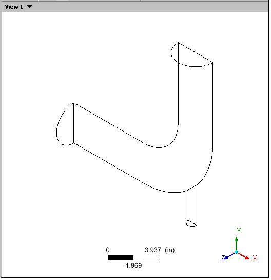
The mixing elbow appears in the 3D Viewer in an isometric orientation. The wireframe appears in the view and there is a check mark beside User Location and Plots > Wireframe in the Outline tree view; the check mark indicates that the wireframe is visible in the 3D Viewer.
Optionally, set the viewer background to white:
Right-click the viewer and select Viewer Options.
In the Options dialog box, select CFD-Post > Viewer.
Set:
Background > Color Type to Solid.
Background > Color to white. To do this, click the bar beside the Color label to cycle through 10 basic colors. (Click the right-mouse button to cycle backwards.) Alternatively, you can choose any color by clicking
 to the right of the Color option.
 Text Color to black (as above).
Edge Color to black (as above).
Click to have the settings take effect.
Experiment with rotating the object by clicking on the arrows of the triad in the 3D Viewer. This is the triad:
In the picture of the triad above, the cursor is hovering in the area opposite the positive Y axis, which reveals the negative Y axis.
Note: The viewer must be in "viewing mode" for you to be able to click the triad. You set viewing mode or select mode by clicking the icons in the viewer toolbar:
When you have finished experimenting, click the cyan (ISO) sphere in the triad to return to the isometric view of the object.
Set CFD-Post to display objects in the units you want to see. These display units are not necessarily the same types as the units in the results files you load; however, for this tutorial you will set the display units to be the same as the solution units for consistency. As mentioned in the Problem Description, the solution units are SI, except for the length, which is measured in inches.
Right-click the viewer and select Viewer Options.
In the Options dialog box, select Common > Units.
Notice that System is set to
SI. In order to be able to change an individual setting (length, in this case) from SI to imperial, set System toCustom. Now set Length to in (inches) and click .
Note:The display units you set are saved between sessions and projects. This means that you can load results files from diverse sources and always see familiar units displayed.
You have set only length to inches; volume will still be reported in meters. To change volume as well, in the Options dialog box, select Common > Units, then click to find the full list of settings.
Optionally, take a few moments to become familiar with the viewer controls. These icons switch the mouse from selecting items in the viewer to controlling the orientation and display of the view. First, the sizing controls:
Click Zoom Box

Click and drag a rectangular box over the geometry.
Release the mouse button to zoom in on the selection.
The geometry zoom changes to display the selection at a greater resolution.
Click Fit View
 to re-center and re-scale the geometry.
Now, the rotation functions:
Click Rotate
 on the viewer toolbar.
 Click and drag repeatedly within the viewer to test the rotation of the geometry. Notice how the mouse cursor changes depending on where you are in the viewer, particularly near the edges:
The geometry rotates based on the direction of movement. If the mouse cursor has an axis (which happens around the edges), the object rotates around the axis shown in the cursor. The axis of rotation is through the pivot point, which defaults to be in the center of the object.
Now explore orientation options:
Right-click a blank area in the viewer and select Predefined Camera > View From -X.
Right-click a blank area in the viewer and select Predefined Camera > Isometric View (Z Up).
Click the "Z" axis of triad in the viewer to get a side view of the object.
Click the three axes in the triad in turn to see the vector objects in all three planes; when you are done, click the cyan (ISO) sphere.
Now explore the differences between the orienting controls you just used and select mode.
Click
 to enter select mode.
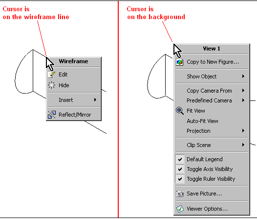
Hover over one of the wireframe lines and notice that the cursor turns into a box.
Click a wireframe line and notice that the details view for the wireframe appears.
Right-click away from a wireframe line and then again on a wireframe line. Notice how the menu changes:
In the Outline tree view, select the elbow1 > fluid > wall check box; the outer wall of the elbow becomes solid. Notice that as you hover over the colored area, the cursor again becomes a box, indicating that you can perform operations on that region. When you right-click the wall, a new menu appears.
Click the triad and notice that you cannot change the orientation of the viewer object. (The triad is available only in viewing mode, not select mode.)
In the Outline tree view, clear the elbow1 > fluid > wall check box; the outer wall of the elbow disappears.
Create an instance reflection on the symmetry plane so that you can see the complete case:
With the 3D Viewer toolbar in viewing mode, click the cyan (ISO) sphere in the triad. This will make it easy to see the instance reflection you are about to create.
Right-click one of the wireframe lines on the symmetry plane. (If you were in select mode, the mouse cursor would have a "box" image added when you are on a valid line. As you are in viewing mode there is no change to the cursor to show that you are on a wireframe line, so you may see the general shortcut menu, as opposed to the shortcut menu for the symmetry plane.) See Figure 2.3: Right-click Menus Vary by Cursor Position.
From the shortcut menu, select Reflect/Mirror. If you see a dialog box prompting you for the direction of the normal, choose the Z axis. The mirrored copy of the wireframe appears.
Tip: If the reflection you create is on an incorrect axis, click
the Undo  toolbar icon twice.
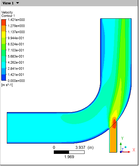
Create a contour plot of velocity on the symmetry plane:
From the menu bar, select Insert > Contour. In the Insert Contour dialog box, accept the default name, and click .
In the details view for
Contour 1, set the following:Click . The contour plot for velocity appears and a legend is automatically generated.
The coloring of the contour plot may not correspond to the colors on the legend because the viewer has a light source enabled by default. There are several ways to correct this:
You can change the orientation of the objects in the viewer.
You can experiment with changing the position of the light source by holding down the Ctrl key and dragging the cursor with the right mouse button.
You can disable lighting for the contour plot. To disable lighting, click the Render tab and clear the check box beside Lighting, then click .
Disabling the lighting is the method that provides you with the most flexibility, so change that setting now.
Click the Z on the triad to better orient the geometry (the 3D Viewer must be in viewing mode, not select mode, to do this).
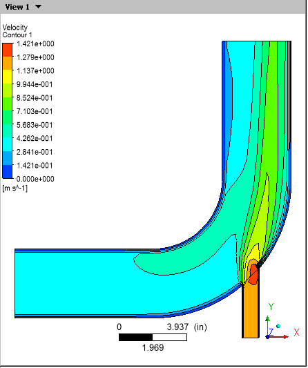
Improve the contrast between the contour regions:
On the Render tab, select Show Contour Lines and click the plus sign to view more options.
Select Constant Coloring.
Set Color Mode to
User
Specified
and Line Color to black (if necessary, click the bar beside Line Color until black appears).Click Apply.
Hide the contour plot by clearing the check box beside User Locations and Plots > Contour 1 in the Outline tree view.
Tip: You can also hide an object by right-clicking on its name in the Outline tree view and selecting Hide.
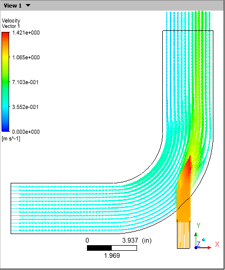
Create a vector plot to show the flow distribution in the elbow:
From the menu bar, select Insert > Vector.
Click to accept the default name. The details view for the vector appears.
On the Geometry tab, set Domains to
fluidand Locations tosymmetry.Click .
On the Symbol tab, set Symbol Size to
4.Click and notice the changes to the vector plot.
Change the vector plot so that the vectors are colored by temperature:
In the details view for Vector 1, click the Color tab.
Set Mode to
Variable.The Variable field becomes enabled.
Click the down arrow
 beside the Variable field
to set it to
beside the Variable field
to set it to Temperature.Click and notice the changes to the vector plot.
Optionally, change the vector symbol. In the details view for the vector, go to the Symbol tab and set Symbol to
Arrow3D. Click .Hide the vector plot by right-clicking on a vector symbol in the plot and selecting Hide.
In this example you will create streamlines to show the flow distribution by velocity and color those streamlines to show turbulent kinetic energy. CFD-Post uses the Variable setting on the Geometry tab to determine how to calculate the streamlines (that is, location). In contrast, the Variable setting on the Color tab determines the color used when plotting those streamlines.
From the menu bar select Insert > Streamline. Accept the default name and click .
In the details view for Streamline 1, choose the points from which to start the streamlines. Click the down arrow
beside the Start From drop-down
widget to see the potential starting points. Hover over each point
and notice that the area is highlighted in the 3D Viewer. It would
be best to show how streamlines from both inlets interact, so, to
make a multi-selection, click Location editor . The Location Selector dialog
box appears.In the Location Selector dialog box, hold down the Ctrl key and click
velocity inlet 5andvelocity inlet 6to select both locations, then click .Click to see the starting points for the streamlines.
On the Geometry tab, ensure that Variable is set to
Velocity.Click the Color tab and make the following changes:
Set Mode to
Variable. The Variable field becomes enabled.Set Variable to
Turbulence Kinetic Energy.Set Range to
Local.
Click . The streamlines show the flow of massless particles through the entire domain.
Select the check box beside Vector 1. The vectors appear, but are largely hidden by the streamlines. To correct this, select
Streamline 1in the Outline tree view and press Delete. The vectors are now clearly visible, but the work you did to create the streamlines is gone. Click the Undo icon to restore Streamline
1.Hide the vector plot and the streamlines by clearing the check boxes beside Vector 1 and Streamline 1 in the Outline tree view.
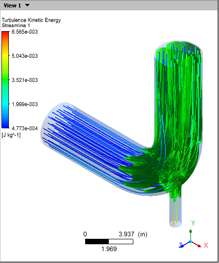
CFD-Post displays vortex core regions to enable you to better understand the processes in your simulation. In this example you will look at helicity method for vortex cores, but in your own work you would use the vortex core method that you find most instructive.
In the Outline tree view:
Under User Locations and Plots, clear the check box for
Wireframe.Under Cases > elbow1 > fluid, select the check box for
wall.Double-click
wallto edit its properties.On the Render tab, set Transparency to
0.75.Click .
This makes the pipe easy to see while also making it possible to see objects inside the pipe.
From the menu bar, select Insert > Location > Vortex Core Region and click to accept the default name.
In the details view for Vortex Core Region 1 on the Geometry tab, set Method to
Absolute Helicityand Level to.01.On the Render tab, set Transparency to
0.2. Click .The absolute helicity vortex that is displayed is created by a mixture of effects from the walls, the curve in the main pipe, and the interaction of the fluids. If you had chosen the vorticity method instead, wall effects would dominate.
On the Color tab, click the colored bar in the Color field until the bar is green. Click .
This improves the contrast between the vortex region and the blue walls.
Right-click in the 3D Viewer and select Predefined Camera > Isometric View (Y up).
In the Outline tree view, select the check box beside Streamline 1. This shows how the streamlines are affected by the vortex regions.
Clear the check boxes beside wall, Streamline 1 and Vortex Core Region 1. Select the check box beside Wireframe.
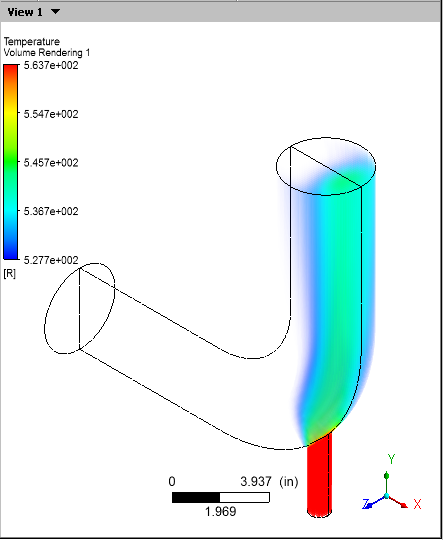
CFD-Post displays volume rendering to enable you to better understand the processes in your simulation.
From the menu bar, select Insert > Volume Rendering and click to accept the default name.
In the details view for Volume Rendering 1 on the Geometry tab, set Variable to
Temperature.On the Color tab, set Mode to
Variableand Variable toTemperature. Click .If necessary to orient the simulation as shown below, right-click in the 3D Viewer and select Predefined Camera > Isometric View (Y up).
Hide the Volume Rendering object by clearing the check box beside Volume Rendering 1 in the Outline tree view.
A contour plot with color bands has discrete colored regions while the display of a variable on a locator (such as a boundary) shows a finer range of color detail by default. The instructions that follow will illustrate a variable at the outlet and create a contour plot that displays the same variable at that same location.
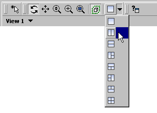
To do the comparison, split the 3D Viewer into two viewports by using the Viewport Layout toolbar in the 3D Viewer toolbar:
Right-click in both viewports and select Predefined Camera > View From -Y.
In the Outline tree view, double-click
pressure outlet 7(which is under elbow1 > fluid). The details view of pressure outlet 7 appears.Click in the View 1 viewport.
In the details view for pressure outlet 7 on the Color tab:
Change Mode to
Variable.Ensure that Variable is set to
Pressure.Ensure that Range is set to
Local.Click . The plot of pressure appears and the legend shows a smooth spectrum that goes from blue to red. Notice that this happens in both viewports; this is because Synchronize visibility in displayed views
 is selected.
Click Synchronize visibility in displayed views
to disable this feature.
Now, add a contour plot at the same location:
Click in View 2 to make it active; the title bar for that viewport becomes highlighted.
In the Outline tree view, clear the check box beside fluid > pressure outlet 7.
From the menu bar, select Insert > Contour.
Accept the default contour name and click .
In the details view for the contour, ensure that Locations is set to
pressure outlet 7and Variable is set toPressure.Set Range to
Local.Click . The contour plot for pressure appears and the legend shows a spectrum that steps through 10 levels from blue to red.
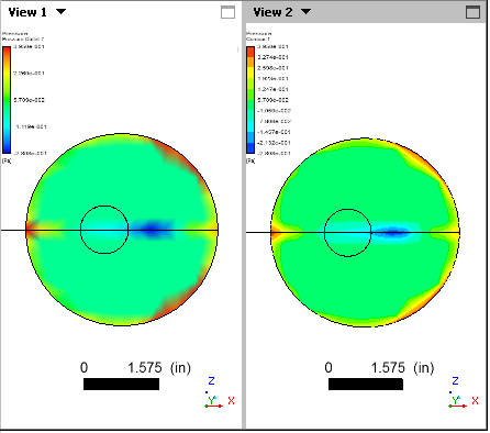
Compare the two representations of pressure at the outlet. Pressure at the Outlet is on the left and a Contour Plot of pressure at the Outlet is on the right:
Enhance the contrast on the contour bands:
In the Outline tree view, right-click User Locations and Plots > Contour 2 and select Edit.
In the details view for the contour, on the Render tab, select Show Contour Lines > Constant Coloring, set Color Mode to
User
Specified
, and click .Click the Labels tab and select Show Numbers. Click .
Explore the viewer synchronization options:
In View 1, click the cyan (ISO) sphere in the triad so that the two viewports show the elbow in different orientations.
In the 3D Viewer toolbar, click Synchronize camera in displayed views
 . Both viewports take the camera
orientation of the active viewport.
. Both viewports take the camera
orientation of the active viewport.Clear the Synchronize camera in displayed views
icon and click the Z arrow head
of the triad in View 1. The object again moves
independently in the two viewports.In the 3D Viewer toolbar, click Synchronize visibility in displayed views
.In the Outline tree view, right-click fluid > wall and select Show. The wall becomes visible in both viewports. (Synchronization applies only to events that take place after you enable the synchronize visibility function.)
When you are done, use the viewport controller to return to a single viewport. The synchronization icons disappear.
As you work, CFD-Post automatically updates a report, which you can see in the Report Viewer. At any time you can publish the report to an HTML file. In this section you will add a picture of the elbow and produce an HTML report:
Click the Report Viewer tab at the bottom of the viewer to view the current report.
In the Outline tree view, double-click the Report > Title Page. In the Title field on the Content tab of the Details of Report Title Page, type:
Analysis of Heat Transfer in a Mixing ElbowClick , then to update the contents of the Report Viewer.
In the Outline tree view, ensure that only User Location and Plots > Contour 1, Default Legend View 1, and Wireframe are visible, then double-click Contour 1. On the Geometry tab, set Variable to
Temperatureand click .On the menu bar, select Insert > Figure. The Insert Figure dialog box appears. Accept the default name and click .
In the Outline tree view, double-click Report > Figure 1. In the Caption field, type
Temperature on the Symmetry
Plane
and click .Click the 3D Viewer, then click the cyan (ISO) sphere in the triad.
Click the Report Viewer tab.
In the top frame of the Report Viewer, click Refresh
 . The report is updated with a picture of the
mixing elbow at the end of the report.
. The report is updated with a picture of the
mixing elbow at the end of the report.Optionally, click to create an HTML version of the report. In the dialog box, click .
The report is written to Report.htm in your working directory.
Right-click in the Outline tree view and select Hide All.
In this section you will generate an expression using the CFX Expression Language (CEL), which you can then use in CFD-Post in place of a numeric value. You will then associate the expression with a variable, which you will also create. Finally, you will create a plane that displays the new variable, then move the plane to see how the values for the variable change.
Define a custom expression for the dynamic head formula (rho|V|^2)/2 as follows:
On the tab bar at the top of the workspace area, select Expressions. Right-click in the Expressions area and select New.
In the New Expression dialog box, type:
DynamicHeadExpClick .
In the Definition area, type in this definition:
Density * abs(Velocity)^2 / 2
where:
Densityis a variableabsis a CEL function (absis unnecessary in this example, it simply illustrates the use of a CEL function)Velocityis a variable
Tip: You can learn which predefined functions, variables, expression, locations, and constants are available by right-clicking in the Definition area.
Click .
Associate the expression with a variable (as the plane you define in the next step can display only variables):
On the tab bar at the top of the workspace area, select Variables. Right-click in the Variables area and select New.
In the New Variable dialog box, type:
DynamicHeadVarClick .
In the details view for DynamicHeadVar, click the drop-down arrow beside Expression and choose
DynamicHeadExp. Click .
Create a plane and animate it:
Click the 3D Viewer tab.
Right-click the wireframe and select Insert > YZ Plane.
If you see a dialog box that asks in which direction you want the normal to point, choose the direction appropriate for your purposes.
A plane that maps the distribution of the default variable (Pressure) appears.
On the Color tab, set Variable to "DynamicHeadVar". On the Render tab, clear Lighting. Click .
The plane now maps the dynamic head distribution.
In the 3D Viewer with the mouse cursor in select mode, click the plane and drag it to various places in the object to see how the location changes the DynamicHeadVar values displayed.
Right-click the plane and select Animate. The Animation dialog box appears and the plane moves through the entire domain, displaying changes to the DynamicHeadVar values as it moves.
In the Animation dialog box, click Stop
 , then click .
Tip: You can define multiple planes and animate them concurrently. First, stop any animations currently running, then create a new plane. To animate both planes, hold down Ctrl to select multiple planes in the Animation dialog box and click Play
 .
.In the upper-left corner of the 3D Viewer, click the down arrow beside Figure 1 and change it to View 1.
In the Outline tree view, right-click User Locations and Plots > Contour 1 and select Hide All.
To this point you have been working with a coarse mesh. In this section you will compare the results from that mesh to those from a refined mesh:
Select File > Load Results. The Load Results File dialog box appears
On the Load Results File dialog box, select Keep current cases loaded and keep the other settings unchanged.
Select
elbow3.cdat.gz(orelbow3.cdat) and click Open.In the 3D Viewer, there are now two viewports: in the title bar for View 1 you have elbow1, and in View 2 you have elbow3. In the Outline tree view under Cases you have elbow1 and elbow3; all boundaries associated with each case are listed separately and can be controlled separately. You also have a new entry: Cases > Case Comparison.
In the Toolbar, select Synchronize camera in displayed views
.If the two cases are not oriented in the same way, clear the Synchronize camera in displayed views
icon and then select it again.
Examine the operation of CFD-Post when the two views are not synchronized and when they are synchronized:
In the viewer toolbar, clear Synchronize visibility in displayed views
.With the focus in View 1, select Insert > Contour and create a contour of pressure on pressure outlet 7 that displays values in the local range.
Note that the contour appears only in View 1. When visibility is not synchronized, changes you make to User Location and Plots settings apply only to the currently active view.
In either view (while in viewing mode), click the Z axis on the triad. Both views show their cases from the perspective of the Z axis.
In the viewer toolbar, select Synchronize visibility in displayed views
.With the focus on the view that contains
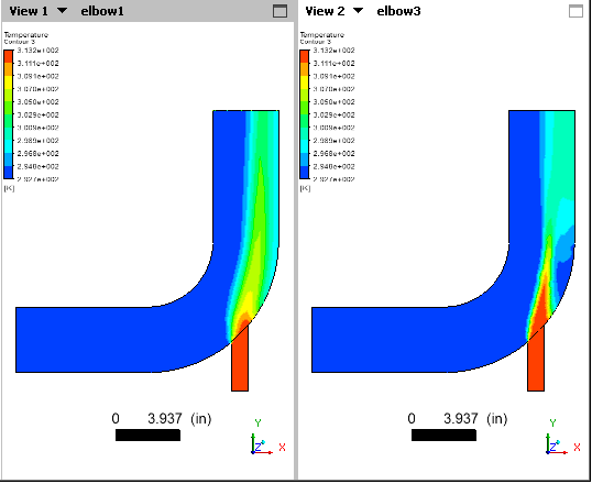
elbow3, select Insert > Contour. Accept the default name and click .Define the contour such that it displays temperature on the symmetry plane:
Tab
Setting
Value
Geometry
Locations
symmetry
Variable
Temperature
Range
Local
Render
Show Contour Bands
> Lighting
(Cleared)
Click Apply.
Note that the contour appears in both views. You can see the differences between the coarse and refined meshes:
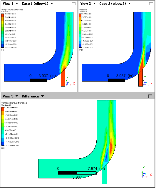
You can now compare the differences between the coarse and refined meshes:
In the Outline tree view, double-click Cases > Case Comparison.
In the Case Comparison details view, select Case Comparison Active and click . The differences between the values in the two cases appear in a third view. Click the Z axis of the triad to restore the orientation of the views.
Now, revert to a single view that shows the original case:
To remove the Difference view, clear Case Comparison Active and click .
To remove the refined mesh case, in the Outline tree view, right-click elbow3 and select Unload.
In the Outline tree view, right-click User Locations and Plots > Contour 1 and select Hide All.
You can export an XML file of Particle Tracks from Fluent and display the tracks in CFD-Post.
To display particle tracks:
With only elbow1.cdat loaded, load the particle track file elbow_tracks.xml:
Select File > Import > Import Fluent Particle Track File.
In the Import Fluent Particle Track File dialog box, select: elbow_tracks.xml
Click .
Click .
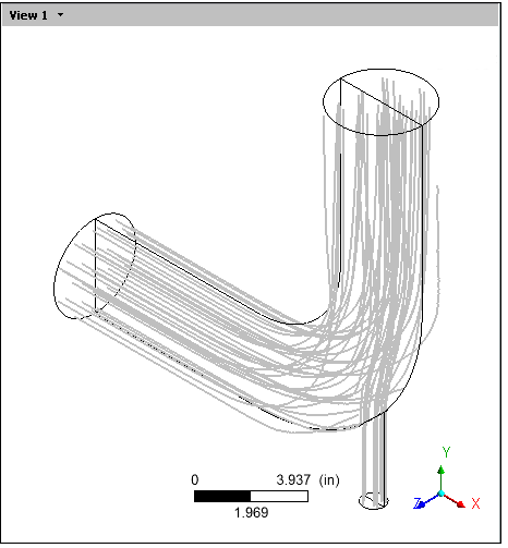
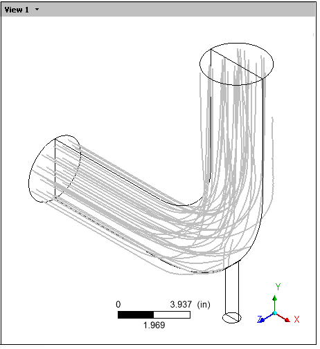
Particle tracks appear in the 3D Viewer. The tracks stretch from the two inlets to the outlet.
Make only the particle tracks from the large inlet visible:
In the Outline tree view, double-click User Locations and Plots> Fluent PT for Anthracite to see the details view for the particle tracks.
In the details view, click the drop-down arrow beside the Injections field so that you can see the names of the two sets of particle tracks.
Select injection-0.
Click .
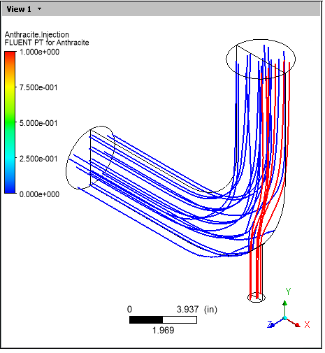
Display both sets of particle tracks, each set in a different color:
First, display both sets of particle tracks again:
Click the drop-down arrow beside the Injections field.
Select injection-0,injection-1.
Click .
Click the Color tab.
Set Mode to
Variable.Set Variable to
Anthracite.Injection.Click .

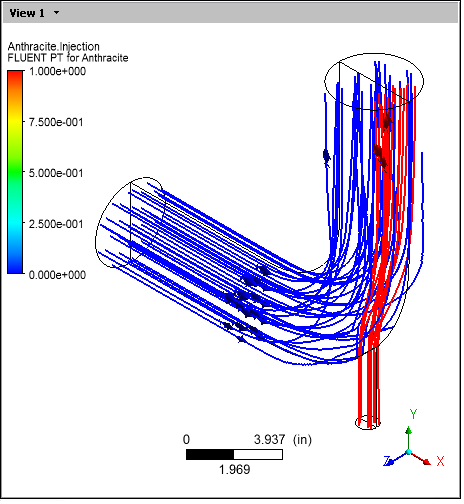
Show fewer particle tracks:
Click the Geometry tab.
Click the drop-down arrow beside the Reduction Type field and select
Reduction Factor.To display only half of the tracks, set Reduction to
2.Click .
Display all tracks again by setting Reduction to
1and clicking .
Animate symbols running along the particle track lines:
Right-click a particle track and select Animate.
The animation begins automatically.
Click Stop the animation
,
then click .On the Options dialog box, set Symbol Size to
2and Symbol toFish3D. Click .In the Animations dialog box, click Play the animation
.
When you have finished viewing the animation, click Stop the animation
, then close the Animation dialog box.
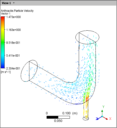
Create a vector plot:
Select Insert > Vector.
In the Insert Vector dialog box, click to accept the default name for the vector.
On the Geometry tab, set:
Locations to
Fluent
PT for Anthracite
Reduction to
Reduction
Factor
Factor to
20Variable to
Anthracite.Particle
Velocity
Tip: You need to click the More Variables
icon to see Anthracite.Particle Velocity.Click the Symbol tab, and set Symbol Size to 2.
Click .
In the Outline tree, clear User locations and Plots > Fluent PT for Anthracite.
After viewing the vector plot, clear User locations and Plots > Vector 2 and select User locations and Plots > Fluent PT for Anthracite in order to view the particle tracks only.
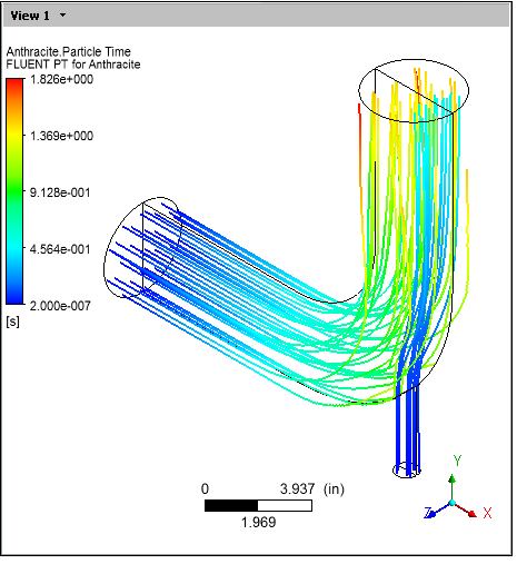
Color the particle tracks by particle time:
Click the Color tab.
Ensure that Mode is set to
Variable.Set Variable to
Anthracite.Particle Time.Click .
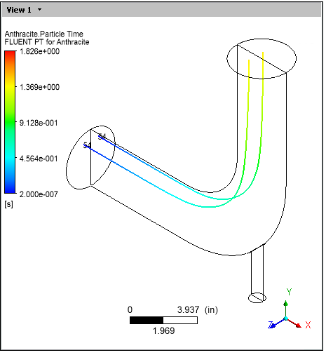
Create a chart of particle time vs. particle velocity Y for a single track:
On the Geometry tab, click the drop-down arrow beside the Injections field and select
injection-0.Click .
On the Symbol tab, select Show Track Numbers and click .
On the Geometry tab:
Enable the Filter option.
Select Track.
In the Track field, type
54.Click .
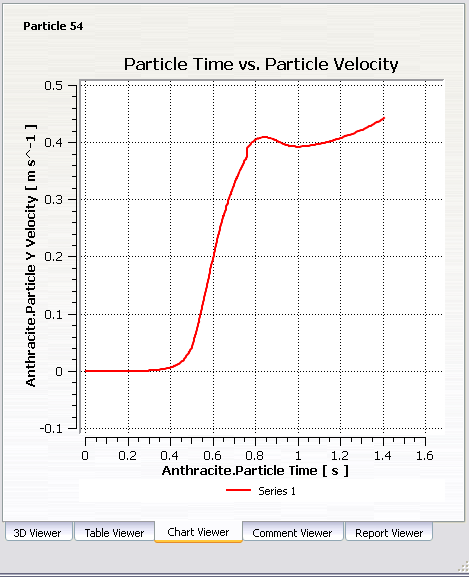
Create a chart of a particle's velocity over time:
From the menu bar, select Insert > Chart.
In the Insert Chart dialog box, type:
Particle 54and click .The details view for the chart appears, and the Chart Viewer appears.
In the Title field, type:
Particle Time vs. Particle VelocityOn the Data Series tab, select
Series 1and set Location toFluent PT for Anthracite.On the X Axis tab, set Variable to
Anthracite.Particle Time.On the Y Axis tab, set Variable to
Anthracite.Particle Y Velocity.Click .
Interpolate a field variable onto the track:
On the tab, set Variable to
Pressure.On the General tab, change the Title to
Particle Time vs. Pressure.Click .
Use the Function Calculator to calculate lengthAve of Pressure on the track:
From the menu bar, select Tools > Function Calculator.
In the Function Calculator, set Function to
lengthAve.Ensure that Location is set to
Fluent PT for Anthracite.Ensure that Variable is set to
Pressure.Enable Show equivalent expression.
Click .
The value of
lengthAve(Pressure)@Fluent PT for Anthraciteappears.
When you began this tutorial, you loaded a solver results file. When you save the work you have done in CFD-Post, you save the current state of CFD-Post into a CFD-Post State file (.cst).
How you save your work depends on whether you are running CFD-Post stand-alone or from within Ansys Workbench:
From CFD-Post stand-alone:
From the menu bar, select File > Save State.
This operation saves the expression, custom variable, and the settings for the objects in a .cst file and saves the state of the animation in a .can file. The .cas.gz and .cdat.gz files remain unchanged.
A Warning dialog box asks if you want to save the animation state. Click .
Optionally, confirm the state file's contents: close the current file from the menu bar by selecting File > Close (or press Ctrl+W) then reload the state file (select File > Load State and choose the file that you saved in step 1.)
From Ansys Workbench:
From the CFD-Post menu bar, select File > Quit. Ansys Workbench saves the state file automatically.
In the Ansys Workbench Project Schematic, double-click the Results cell. CFD-Post re-opens with the state file loaded.
Save a picture of the current state of the simulation: In the Outline tree view, show Contour 1. With the focus in the 3D Viewer, click Save Picture
 from the toolbar. In the Save Picture dialog box, click . A PNG file of the
current state of the viewer is saved to
from the toolbar. In the Save Picture dialog box, click . A PNG file of the
current state of the viewer is saved to <casename>.png (elbow1.png) in your working directory.You can recreate the animation you made previously and save it to a file:
Click the cyan (ISO) sphere in the triad to orient the elbow to display Plane 1.
In the Outline tree view, clear Contour 1 and Fluent PT for Anthracite; show Plane 1.
Right-click Plane 1 in the 3D Viewer and select Animate. The Animation dialog box appears and the plane moves through the entire domain.
Click the stop icon
.If necessary, display the full animation control set by clicking
 .
. 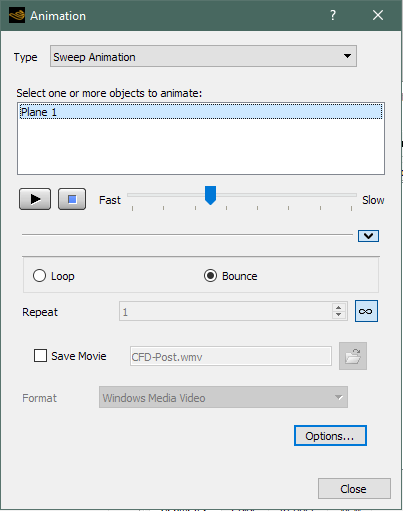
The Repeat is set to infinity; change the value to 1 by clicking the infinity button. The Repeat field becomes selected and by default is set to one.
Select Save Movie to save the animation to the indicated file.
Click Play the animation
.The plane moves through one cycle.
You can now go to your working directory and play the animation file in an appropriate viewer.
Click to close the Animation dialog box.
Close CFD-Post: from the toolbar select File > Quit. If prompted, you may save your changes.
As you worked through this tutorial you generated the following files in your working directory (default names are given):
elbow1.cst, the state file, and elbow1.can, the animation associated with that state file
elbow1.wmv, the animation
elbow1.png, a picture of the contents of the 3D Viewer
Report.htm, the report.