

This tutorial demonstrates the quantitative postprocessing capabilities of CFD-Post using a 3D model of a circuit board with a heat-generating electronic chip mounted on it. The flow over the chip is laminar and involves conjugate heat transfer.
The heat transfer involves conduction in the chip and conduction and convection in the surrounding fluid. The physics of conjugate heat transfer such as this is common in many engineering applications, not just the design and cooling of electronic components.
In this tutorial, you will read the case and data files and perform a number of postprocessing exercises.
This tutorial demonstrates how to do the following:
Note: These tutorials are prepared on a Windows system. The screen shots in the tutorials may be slightly different than the appearance on your system, depending on the operating system or graphics card.
The problem is shown schematically in Figure 4.1: Problem Specification. The configuration consists of a series of side-by-side electronic chips, or modules, mounted on a circuit board. Air flow, confined between the circuit board and an upper wall, cools the modules. To take advantage of the symmetry present in the problem, the model will extend from the middle of one module to the plane of symmetry between it and the next module.
As shown in the figure, each half-module is assumed to generate 2.0 Watts and to have a bulk conductivity of 1.0 W/m2K. The circuit board conductivity is assumed to be one order of magnitude lower: 0.1 W/m2K. The air flow enters the system at 298 K with a velocity of 1 m/s. The Reynolds number of the flow, based on the module height, is about 600. The flow is therefore treated as laminar.

If this is the first tutorial you are working with, it is important to review Introduction to the Tutorials before beginning.
Create a working directory.
CFD-Post uses a working directory as the default location for loading and saving files for a particular session or project.
Download the
quantitative.zipfile here .Unzip
quantitative.zipto your working directory.Ensure that the following tutorial input files are in your working directory:
chip.cas.gz
chip.cdat.gz
Before you start CFD-Post, set the working directory. The procedure for setting the working directory and starting CFD-Post depends on whether you run CFD-Post stand-alone, from the Ansys CFX Launcher, or from Ansys Workbench:
To run CFD-Post stand-alone
On Windows:
From the Start menu, right-click All Programs > ANSYS 2024 R2 > Fluid Dynamics > CFD-Post 2024 R2 and select Properties.
Type the path to your working directory in the Start in field and click .
Click All Programs > ANSYS 2024 R2 > Fluid Dynamics > CFD-Post 2024 R2 to launch CFD-Post.
On Linux, enter
cfdpostin a terminal window that has its path set up to run CFD-Post. The path will be something similar to/usr/ansys_inc/v242/CFD-Post/bin.
To run Ansys CFX Launcher
Start the launcher.
You can run the launcher in any of the following ways:
On Windows:
From the Start menu, select All Programs > ANSYS 2024 R2 > Fluid Dynamics > CFX 2024 R2.
In a Command Prompt that has its path set up correctly to run CFX, enter
cfx5launch. If the path is not set up correctly, you will need to type the full pathname of thecfxcommand, which will be something similar toC:\Program Files\ANSYS Inc\v242\CFX\bin.
On Linux, enter
cfx5launchin a terminal window that has its path set up to run CFX .The path will be something similar to/usr/ansys_inc/v242/CFX/bin.
Set the working directory.
Click the CFD-Post 2024 R2 button.
Ansys Workbench
Start Ansys Workbench.
From the menu bar, select File > Save As and save the project file to the directory that you want to be the working directory.
Open the Component Systems toolbox and double-click Results. A Results system opens in the Project Schematic.
Right-click the A2 Results cell and select Edit. CFD-Post opens.
In the steps that follow, you will explore the solution using CFD-Post.
Before you perform various quantitative analyses of the case, prepare the case and CFD-Post:
Start CFD-Post now and load the CDAT file (chip.cdat.gz) from the menu bar by selecting > . In the Load Results File dialog box, select chip.cdat.gz and click .
Set CFD-Post to display the units you want to see. These display units are not necessarily the same types as the units in the results files you load; however, for this tutorial you will set the display units to be the same as the solution units.
Right-click the viewer and select Viewer Options.
In the Options dialog box, select Common > Units.
Set System to
SIand click .
Note: The display units you set are saved between sessions and projects. This means that you can load results files from diverse sources and always see familiar units displayed.
Optionally, set the viewer background to white:
Right-click the viewer and select Viewer Options.
In the Options dialog box, select CFD-Post > Viewer.
Set:
Background > Color Type to Solid.
Background > Color to white. To do this, click the bar beside the Color label to cycle through 10 basic colors. (Click the right-mouse button to cycle backwards.) Alternatively, you can choose any color by clicking
 icon to the right of the Color option.
 Text Color to black (as above).
Edge Color to black (as above).
Click to have the settings take effect.
There are two ways to view the mesh: you can use the wireframe for the entire simulation or you can view the mesh for a particular portion of the simulation.
To view the mesh for the entire simulation:
Right-click a line of the wireframe in the 3D Viewer and select Show surface mesh to display the mesh.
Click the "Z" axis of triad in the viewer to get a side view of the object.
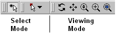
Note: The 3D Viewer toolbar has to be in viewing mode for you to be able to select the triad elements.
In the Outline tree view, double-click User Locations and Plots > Wireframe to display the wireframe's editor.
Tip: Click the Details of Wireframe editor and press F1 to see help about the Wireframe object.
On the Wireframe details view, click and to restore the original settings.
To view the mesh for a particular portion of the simulation (in this case, the chip (wall 4 shadow)):
In the Outline tree view, select the check box beside Cases > chip > fluid 8 > wall 4 shadow, then double-click wall 4 shadow to edit its properties in its details view.
In the details view:
On the Render tab, clear Show Faces.
Select Show Mesh Lines.
Ensure that Edge Angle is set to 0 [degree].
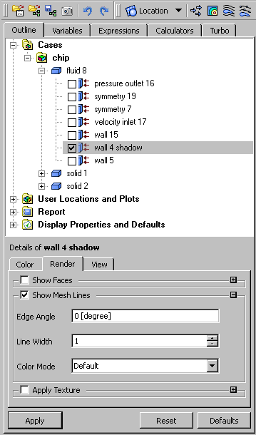
Click .
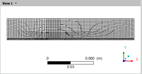
The mesh appears and is similar to the mesh shown by the previous procedure, except that the mesh is shown only on the chip.
Now, clear the display of the chip wireframe. In the details view:
Clear Render > Show Mesh Lines.
Select Show Faces.
Click .
The chip reappears.
In the Outline tree view, clear the check box beside Cases > chip > fluid 8 > wall 4 shadow.
To check the mesh:
Select the Calculators tab at the top of the workspace area, then double-click Mesh Calculator. The Mesh Calculator appears.
Using the drop-down arrow beside the Function field, select a function such as
Maximum Face Angle.
Click . The results of the calculation appear.
Repeat the previous steps for other functions, such as
Mesh Information.
You can view values in the simulation by using the Function Calculator:
In the Calculators view, double-click Function Calculator. The Function Calculator appears.
In the Function field, select
minValas the function to evaluate.In the Location field, select
wall 4.Beside the Variable field, select
Xin the Variable Selector dialog box.Clear the Clear previous results on calculate setting and select Show equivalent expression.
Click to see the result of the calculation of the minimum X value of the chip.
Repeat the operation, but in the Function field, select
maxValas the function to evaluate. Click to see the result of the calculation of the maximum X value of the chip.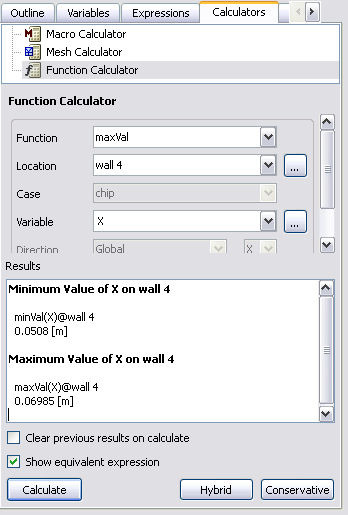
You will use these values in subsequent steps.
Lines can be used to display quantitative results of your CFD simulations. Here, you will create a line along which to plot the temperature distribution along the top center of the chip.
Select > > .
For the name, type
topcenterlineand click .On the Details of topcenterline > Geometry tab:
Set Method to
Two Points.Set Point 1 to
0.0508,0.01,0.Set Point 2 to
0.06985,0.01,0.Ensure that Line Type is set to
Sample.
Those coordinates define a line along the top center of the chip.
On the Color tab:
Set Mode to
Variable.Set Variable to
Temperature.
These steps will color the line by temperature and cause the legend to be displayed.
Click .

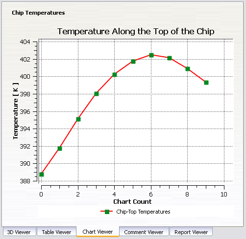
Here you will plot the temperature distribution along a line along the top center of the chip.
Select > .
For the name, type
Chip Temperaturesand click .The Details of Chip Temperatures view appears.
On the General tab:
Set Title to
Temperature Along the Top of the Chip.Set Caption to
Graph
of the Temperature Along the Top of the Chip
.
On the Data Series tab
Set Location to
topcenterline.Change the name
Series 1toChip-Top Temperatures.
On the X Axis tab, set Variable to
Chart Count.On the Y Axis tab, set Variable to
Temperature.On the Line Display tab, select Chip-Top Temperatures and set Symbols to
Rectangle.Make the Symbol Color a darker shade of green: beside the Symbol Color field, click Color Selector
 , select a new shade of green, and
click .
, select a new shade of green, and
click .Click .
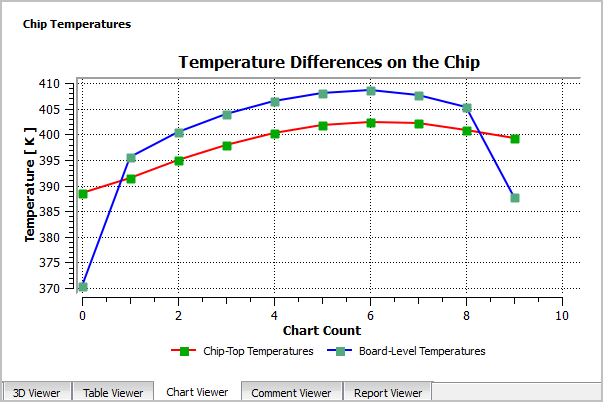
Here you will create a second line near the bottom of the chip so that you can compare that to the temperature distribution along the top center of the chip.
Select > > .
For the name, type
bottomsidelineand click .On the Details of bottomsideline > Geometry tab:
Set Method to
Two Points.Set Point 1 to
0.0508,0.0027,0.Set Point 2 to
0.06985,0.0027,0.Set Line Type to
Sample.
Those coordinates define a line near board level beside the chip.
Click .
Here you will plot the temperature distribution along the second line.
In the area of the Tree view, double-click .
On the General tab, change Title to
Temperature Differences on the Chipand Caption toGraph of the Temperature Along the Top and Bottom of the Chip.On the Data Series tab:
Click New
 to
create
to
create Series 2.Set Location to
bottomsideline.Change the name
Series 2toBoard-Level Temperatures.
On the Line Display tab, select Board-Level Temperatures and set Symbols to
Rectangle.Beside the Symbol Color field, click Color Selector
, select a new shade of green, and
click .Click .
You can create a table to show how values change at different locations, provided that the locations have been defined. In this section you will create three planes along the mixing region and measure the temperatures on those planes. You will then create a table and define functions that show temperature minimums and maximums, and the differences between those values.
In the 3D Viewer, ensure that only the wireframe is visible.
Click the cyan-colored ball on the triad to make it easier for you to see the temperature planes that you will create.
From the toolbar, select Location > Plane. In the Insert Plane dialog box, type
Table Plane 1and click .In the details view for Table Plane 1, set the following values:
Tab
Field
Value
Geometry
Domains
fluid 8
Definition
> Method
YZ Plane
Definition
> X
0.051 [m]
Color
Mode
Variable
Variable
Temperature
Range
Local
Render
Lighting
(Cleared)
Click .
Right-click Table Plane 1 and select Duplicate. The Duplicate dialog box appears.
In the Duplicate dialog box, accept the default name
Table Plane 2and click .In the Outline tree view, double-click Table Plane 2 and on the Geometry tab change Definition > X to 0.0605. Click .
Repeat the previous step, duplicating
Table Plane 2to makeTable Plane 3and changing Definition > X to 0.0697. Click .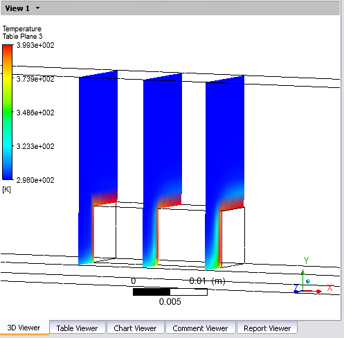
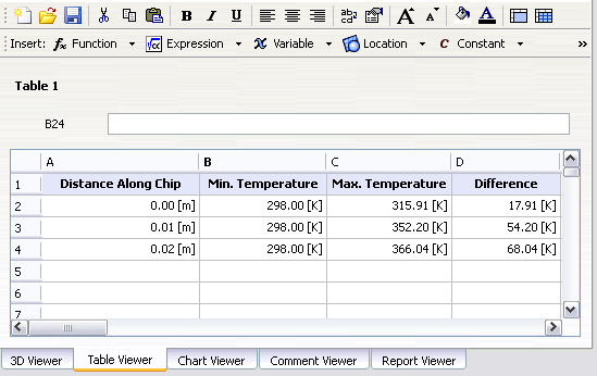
Now, create a table:
From the menu bar, select Insert > Table. Accept the default table name and click .
The Table Viewer opens.
Type in the following headings:
A
B
C
D
1
Distance Along Chip
Min. Temperature
Max. Temperature
Difference
For the "Distance Along Chip" column, create an equation that gives the distance from the beginning of the chip (which is available from "wall 4" in "solid 2"). Click cell A2, then in the Table Viewer's Insert bar, select Function > CFD-Post > minVal. In the cell definition field you see
=minVal()@, which will be the base of the equation. With the cursor between the parentheses, typeX. Move the cursor after the@sign and either typeTable Plane 1or select Insert > Location > Table Plane 1.=minVal(X)@Table Plane 1 - minVal(X)@wall 4
When you click away from cell A2, the equation is solved.
Note: The expressions in the equation are what you created in the Function Calculator. You can copy expressions from the Function Calculator and paste them into table cells, adding other characters in the cell definition field as required.
Complete the rest of the table by entering the following cell definitions:
- Cell A2
=minVal(X)@Table Plane 1 - minVal(X)@wall 4
- Cell A3
=minVal(X)@Table Plane 2 - minVal(X)@wall 4
- Cell A4
=minVal(X)@Table Plane 3 - minVal(X)@wall 4
- Cell B2
=minVal(T)@Table Plane 1
- Cell B3
=minVal(T)@Table Plane 2
- Cell B4
=minVal(T)@Table Plane 3
- Cell C2
=maxVal(T)@Table Plane 1
- Cell C3
=maxVal(T)@Table Plane 2
- Cell C4
=maxVal(T)@Table Plane 3
- Cell D2
=maxVal(T)@Table Plane 1 - minVal(T)@Table Plane 1
- Cell D3
=maxVal(T)@Table Plane 2 - minVal(T)@Table Plane 2
- Cell D4
=maxVal(T)@Table Plane 3 - minVal(T)@Table Plane 3
As you complete the table, notice that the minimum temperature values stay constant, but the maximum values increase as the chip heats the passing air.
The default format for cell data is appropriate for some variables, but it is not appropriate here. Click cell A2, then while depressing the Shift key, click in the lower-right cell (D4). Click the Number Formatting
 icon in the Table Viewer toolbar. In the Cell Formatting dialog box, set Precision to
 2, change Scientific toFixed, and click .Optionally, apply some formatting to the table.
You can view the table in three places: in the Table Viewer (where you can apply formatting), in the Report Viewer (where some of the formatting you applied in the Table Viewer will be visible), and in the published report (which has default formatting for tables that you cannot see in either the Table Viewer or the Report Viewer, but which are overridden by any formatting changes you make in the Table Viewer). It is useful to view the published report (see Publish a Report) before applying formatting in the Table Viewer.
To format the table as shown above:
For cells A1-D1: Apply bold font, background color, and text centering. Manually resize cell widths individually.


For cells A2-D4: Right-justified text.

To save a report as an HTML file:
Click the Report Viewer tab.
Click at the top of the Report Viewer.
In the dialog box, specify a meaningful name for the report, such as
IC_Cooling_Simulation.htm.Tip: Click the Browse icon in the dialog box to control where the report is stored.
Click .