The following turbo charts are available:
The Blade Loading feature plots pressure (or another chosen variable) on the blade at a given spanwise location. A polyline is created at the given spanwise location.
A special variable, Streamwise (0-1) is
available as the X Variable used in blade loading
plots. This is a streamwise coordinate that follows the blade surface;
it can be used as a substitute for the axial coordinate (for example, X) or the variable Chart Count. The
streamwise coordinate is based on the meridional coordinate, and is
normalized so that it ranges from 0 at the leading edge to 1 at the
trailing edge of the blade.
Select a streamwise and spanwise location and a number of sampling points.
Note: The Theta extents of the chart line are set to the Theta
extents of the domain or, in the case of data instancing, the Theta
extents of the expanded set of domains. Some of the sample points
may fall outside the domain. To see the circumferential chart line,
edit the Plots > 3D View object and turn on Show chart location lines.
Hub to Shroud has the following options:
- 15.7.6.3.1. Single Line vs. Two Lines
- 15.7.6.3.2. Display
- 15.7.6.3.3. Mode
- 15.7.6.3.4. Point Type
- 15.7.6.3.5. Theta
- 15.7.6.3.6. Samples
- 15.7.6.3.7. Streamwise
- 15.7.6.3.8. Distribution
- 15.7.6.3.9. X/Y Variable
- 15.7.6.3.10. Circumferential Averaging by Length: Hub to Shroud Turbo Chart
- 15.7.6.3.11. Circumferential Averaging by Area: Hub to Shroud Turbo Chart
- 15.7.6.3.12. Circumferential Averaging by Mass Flow: Hub to Shroud Turbo Chart
- 15.7.6.3.13. Constant Blade Aligned Linear Coordinates
- 15.7.6.3.14. Constant Blade Aligned Coordinates
Select either Single Line or, to perform
a comparison between two streamwise locations on a hub-to-shroud plot,
to Two Lines.
If you have selected Two Lines, you can
set Display to:
Separate LinesDisplays the two lines without performing any comparisons.
Difference (S2–S1)Displays the difference in the circumferentially averaged variable between the two locations, relative to the first line’s location.
Ratio (S2/S1)Displays the ratio of the difference in the circumferentially averaged variable between the two locations, relative to the first line’s location.
When Display is set to Difference
(S2–S1) or Ratio (S2/S1), you
can set the Compare option to X Values or to Y Values. The selected values will be
compared between the two lines.
Set Mode to one of the following options:
Two Points LinearThe
Two Points Linearoption causes the hub-to-shroud line to be a straight line, specified by two points: one on the hub and one on the shroud. The Point Type setting (described below) specifies the coordinate system for interpreting the specified points.Blade Aligned LinearThe
Blade Aligned Linearoption causes the hub-to-shroud line to be specified by a curve of constant Linear BA Streamwise Location coordinate. For details, see Constant Blade Aligned Linear Coordinates.Blade AlignedThe
Blade Alignedoption causes the hub-to-shroud line to be specified by a curve of constant BA Streamwise Location coordinate. For details, see Constant Blade Aligned Coordinates.Streamwise LocationThe
Streamwise Locationoption causes the hub-to-shroud line to be specified by a curve of constant streamwise coordinate. Here, the streamwise coordinate system is derived from a "background mesh". For details, see Background Mesh Frame.
Note:
Blade Aligned coordinates may not always be available, depending on the case geometry. In particular, if the blade tip clearance is large or uneven between the leading and trailing edges, CFD-Post may not be able to detect the blade edge lines. In this case you will not be able to use Blade Aligned coordinates in turbo surface or turbo chart specification.
In turbo line, turbo surface, and related editors, the Blade Aligned coordinate values that you enter in the input fields (and the related CCL parameters) are normalized to the blade's leading and trailing edge locations with predefined constant references: 0.25 and 0.75 are taken to be the blades leading and trailing edges, respectively. The normalization of the input values is to enable a consistent reference to the leading and trailing edges regardless of specific cases. These values are conventions, not real blade aligned coordinated values; the normalized values are translated by the engine to create the real Blade Aligned coordinate values before constructing turbo lines and turbo surfaces.
The Point Type setting is applicable when Mode is set to Two Points Linear.
It controls the coordinate system for defining the specified hub and
shroud point coordinates. The options for Point Type are:
ARWhen the
ARoption is selected, the hub and shroud points are specified in AR (axial, radial) coordinates.XYZWhen the
XYZoption is selected, you specify the x, y, and z coordinates of the line's end points.Blade Aligned LinearWhen the
Blade Aligned Linearoption is selected, the hub and shroud points are specified, each by a single Linear BA Streamwise Location coordinate. For details, see Constant Blade Aligned Linear Coordinates.Streamwise LocationWhen the
Streamwise Locationoption is selected, the hub and shroud points are specified, each by a single streamwise coordinate. Here, the streamwise coordinate system is derived from a "background mesh". For details, see Background Mesh Frame.
The Theta setting is available with the Hub to Shroud methods.
The Samples setting controls the number of sampling points between the hub and shroud.
The Streamwise field sets the streamwise location for a chart line.
When Display is set
to Difference or Ratio,
the Streamwise fields set the
locations to compare.
Note: When there is a domain interface at a single streamwise location, for example a domain interface between the rotor and stator domains of a compressor stage, choosing a streamwise location exactly on the interface might lead to unexpected results. To cause CFD-Post to sample values from the intended side of the interface, choose a streamwise position slightly away from the interface. For example, if there is an interface at a streamwise position of 1, you could set Streamwise to 0.99999 or 1.00001 to cause CFD-Post to sample values from one side or the other.
Each sampling point value is evaluated from a corresponding circular band. The Distribution setting controls how the sampling points and their corresponding bands are distributed from hub to shroud (at the same streamwise coordinate).
The Distribution options are:
Equal
Distance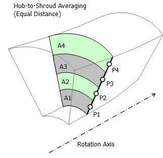
The
Equal Distanceoption (default) causes the sampling points to be distributed at uniform distances along a hub-to-shroud path. For circumferential averaging purposes, contiguous circular bands are internally constructed, one for each sampling point, concentric about the rotation axis, width-centered (in the spanwise direction) about each sampling point, each band having the same width or spanwise extent.Equal Mass Flow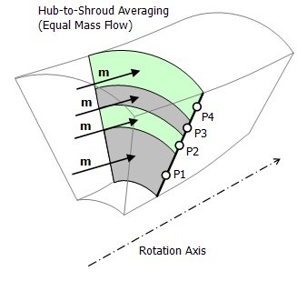
The
Equal
Mass Flow
option causes the sampling points to be distributed along a hub-to-shroud path such that contiguous circular bands can be internally constructed, one for each sampling point, concentric about the rotation axis, width-centered (in the spanwise direction) about each sampling point, with an equal mass flow through each band (except possibly the first and last bands). See Include Boundary Points, below.Note: CFD-Post cannot create an Equal Mass Flow point distribution for some cases:
When there is a cross-section recirculation and the total mass flow on the section is near zero, the point distribution will fail.
When there is a mass flow 'spike' on the section (usually this is caused by an ill-defined solution), the equal mass distribution will be impractical.
When too many sample points are requested over a small area.
Equal
Area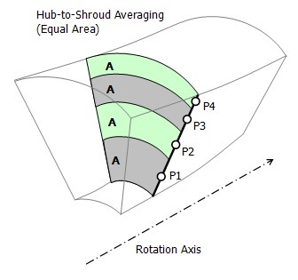
The
Equal Areaoption causes the sampling points to be distributed along a hub-to-shroud path such that contiguous circular bands can be internally constructed, one for each sampling point, concentric about the rotation axis, width-centered (in the spanwise direction) about each sampling point, with an equal area for each band (except possibly the first and last bands). See Include Boundary Points, below.Mesh Density Based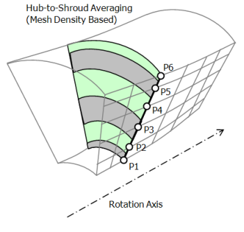
The
Mesh Density
Based
option causes the sampling points to be distributed along a hub-to-shroud path such that the sampling point density is proportional to the mesh node density along eitherthe intersection of the inlet with the periodic surface, or
the intersection of the outlet with the periodic surface,
whichever of these paths has a greater number of nodes.
The following settings are available:
Max. Number of Points > Max. Points
The Max. Points setting controls the number of points of analysis.
Reduction Factor > Factor
The Factor setting specifies the ratio of mesh nodes to sampling points along the hub-to-shroud path. A value of 1 causes one sampling point to be created per mesh node. You can reduce the computational time by setting a larger reduction factor.
Note: For Two-Line Hub to Shroud plots, you may not be able to create Difference and Ratio plots using Reduction Factor if the two lines are in different domains.
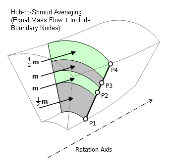
When Distribution is set to Equal
Mass Flow or Equal Area, the Include Boundary Points option is available. This option
shifts all of the bands so that the first and last sampling points
are on the hub and shroud. The first and last bands are then "half"
the size of the other bands (in terms of the particular measure used
in the band construction: distance, mass flow, or area). See Figure 15.1: Sampling Point Distribution with Include Boundary Nodes Option.
When the Circ. Average setting is set to Length, circumferential averaging of values at a sampling
point is carried out internally by forming a circular arc, centered
about the rotation axis, passing through the sampling point. Values
are interpolated to n equally-spaced locations
along the arc, using values from nearby nodes, where n is a number that is inversely proportional to the mesh length scale,
and limited by the Max. Samples setting. The n values are then averaged in order to obtain a single,
circumferentially-averaged value for the sampling point.

When the Circ. Average setting is set to Area, a variable value at each sampling point is calculated
as an area average over the corresponding circular band that was internally
constructed as part of the process of distributing the sampling points.
For details, see Distribution.
When the Circ. Average setting is set to Mass, a variable value at each sampling point is calculated
as a mass flow average over the corresponding circular band that was
internally constructed as part of the process of distributing the
sampling points. For details, see Distribution.
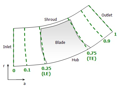
The Constant Blade Aligned Linear coordinates
are defined as 0 (zero) at the inlet, 0.25 at a straight line that
approximates the blade leading edge, 0.75 at a similar line for the
trailing edge, and 1.0 at the outlet, adding 1.0 for each successive
turbomachinery component downstream of the first. Dashed lines in Figure 15.3: Blade Aligned Linear Coordinates show
constant values of Constant Blade Aligned Linear coordinate.
For more details on the convention that 0.25 and 0.75 are taken to be the blades leading and trailing edges, see Mode.
The Constant Blade Aligned coordinates
are defined as 0 (zero) at the inlet, 0.25 at the blade leading edge,
0.75 at the trailing edge, and 1.0 at the outlet, adding 1.0 for each
successive turbomachinery component downstream of the first.
For more details on the convention that 0.25 and 0.75 are taken to be the blades leading and trailing edges, see Mode.

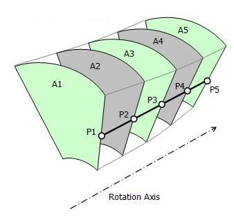
The distance between sampling points between the inlet and outlet is controlled by the number you enter in the Samples box. Choose X and Y variables for the chart axes from the list.
When the Circ. Average setting is set to Length, circumferential averaging of values is carried
out internally by creating arcs through sampling about the rotation
axis. Values are interpolated to n equally-spaced locations along
the arc, using values from nearby nodes, where n is a number that
is inversely proportional to the mesh length scale, and limited by
the Max. Samples setting. The n values are then averaged in order
to obtain a single, circumferentially-averaged value for the sampling
point.
When performing area average or mass-flow average calculations, surfaces of constant-streamwise coordinate are used to carry out the averaging. Each surface passes through its associated sampling point, as shown in Figure 15.5: Inlet to Outlet Sample Points.