


To create and view a chart object:
Click Create Chart
 or select Insert > Chart.
The Insert Chart dialog box appears.
Enter a name for the new chart object.
Click .
The chart object appears under the Report heading in the tree view. A details view appears for the new chart object and the Chart Viewer takes focus.
Edit the chart settings as appropriate for each tab:
Click to see the results of your changes displayed in the Chart Viewer.
Optionally, on the Data Series tab click the Get Information on the Item icon
 to view summary data for the current series.
Optionally, click to save the chart data in a Comma Separated Values (CSV) file. You can load the values in the CSV file into external programs such as Microsoft Excel.
To see the chart in the report, you must generate the report as described in Report.
The General tab is used to define the chart type, the main title, and the report caption.
The Type setting has the following options:
| Option | Description |
|---|---|
|
| Plots X axis variable vs. the Y axis variable. XY - Line charts use polyline or line locators to plot values that vary in space. |
|
| Plots X axis variable vs. the Y axis variable. XY - Scatter charts use symbols to represent the X-axis and Y-axis variable values for each point in the selected location. |
|
| Plots an Expression (typically time) on the X axis and enables you to specify a variable to plot on the Y axis. Transient or Sequence charts use expressions or a point locator to plot the variation of a scalar value vs. time. |
|
| Plots the number of values or the proportion of values that fall into each specified category. |
The Title setting specifies a title for the Chart object. Clear the Display Title check box if you don’t require a chart title.
The Caption is the description of the Chart object that appears in the report.
The Fast Fourier Transform check box can be selected only for Transient or Sequence charts. When the Fast Fourier Transform check box is selected, the following options are available:
- Modify Input Signal Filter
Enables you to select the signal filter to be
Hanning(default),Barlett,Blackman,Hamming, orNone. For details, see Fast Fourier Transform (FFT) Theory.- Subtract mean
Causes the mean to be subtracted from each value to better show the amplitude of the noise.
Note: This feature applies to all loaded files.
- Full range of input data vs. Setting Min/Max Limits
You can choose to analyze the Full range of input data or to set Min and Max values. To get the range for the Min and Max values, click Get range from FFT output
 .
.- Reference Values
Click to display the Reference Values dialog box. There you can set the following values (which will apply to all Fast Fourier Transform charts): Reference Acoustic Pressure, Length, Velocity, and whether to Save as default.
When interpreting time-sequence data from a transient solution, it is often useful to look at the data's frequency attributes. For instance, you may want to determine the major vortex-shedding frequency from the time-history of the drag force on a body recorded during a simulation, or you may want to compute the frequency distribution of static pressure data recorded at a particular location on a body surface. Similarly, you may need to compute the frequency distribution of turbulent kinetic energy using data for fluctuating velocity components.
To interpret some of these time-dependent data, you need to perform Fourier transform analysis. The Fourier transform enables you to take any time-dependent data and resolve it into an equivalent summation of sinusoids.
The CFD-Post FFT module assumes that the input data have been sampled at equal intervals and are consecutive (in the order of increasing time).
The lowest non-zero frequency that the FFT module can pick up,  , is given by
  , where
  is the total number of samples, and
  is the sampling interval (or timestep size). If
the sampled sequence contains frequencies lower than this, these frequencies
will be aliased into higher frequencies.
is the sampling interval (or timestep size). If
the sampled sequence contains frequencies lower than this, these frequencies
will be aliased into higher frequencies.
The highest frequency that the FFT module can pick up,  , is given by
  . Note that the floor
function has been applied to
. Note that the floor
function has been applied to  to
round it down to the nearest integer. Note that, when
to
round it down to the nearest integer. Note that, when  is even,
  .
.
The value at zero frequency represents the mean value. The mean value can be taken out of the plot by selecting Subtract mean check box.
The discrete FFT algorithm is based on the assumption that the time-sequence data passed to the FFT corresponds to a single period of a periodically repeating signal. Because in most situations the first and the last data points will not coincide, the repeating signal implied in the assumption can have a large discontinuity. The large discontinuity produces high-frequency components in the resulting Fourier modes, causing an aliasing error. You can condition the input signal before the transform by "windowing" it, in order to avoid this problem.
Suppose there are  consecutive
discrete (time-sequence) data that are sampled with a constant interval
consecutive
discrete (time-sequence) data that are sampled with a constant interval  :
:
 | (12–43) |
Windowing is done by multiplying the original input data ( ) by a window function
  :
:
 | (12–44) |
There are four different window functions:
Hamming's window:
 | (12–45) |
Hanning's window:
 | (12–46) |
Barlett's window:
 | (12–47) |
Blackman's window:
 | (12–48) |
These window functions preserve 3/4 of the original data, affecting only 1/4 of the data the ends.
The Fourier transform utility enables you to compute the Fourier
transform of a signal,  , a real-valued function, from a finite
number of its sampled points.
, a real-valued function, from a finite
number of its sampled points.
For a periodic set of  sampled points,
  , the discrete Fourier transform expresses the signal
as a finite trigonometric series:
, the discrete Fourier transform expresses the signal
as a finite trigonometric series:
 | (12–49) |
where the series coefficients  are computed as
 | (12–50) |
The previous two equations form a Fourier transform pair that enables you to determine one from the other.
Note that when you vary  from
0 to
from
0 to  in Equation 12–49 or Equation 12–50, the following is true:
 and
and  form a complex conjugate
pair.
form a complex conjugate
pair.The value at
 is unique and
corresponds to zero frequency.
is unique and
corresponds to zero frequency.When
 is even, the range of index
  corresponds to positive frequencies,
and the range of index
corresponds to positive frequencies,
and the range of index  corresponds to negative frequencies. The frequency
at
corresponds to negative frequencies. The frequency
at  , called
the Nyquist frequency, is a unique value.
, called
the Nyquist frequency, is a unique value.When
 is odd, the range of index
  corresponds to positive frequencies,
and the range of index
corresponds to positive frequencies,
and the range of index  corresponds to negative frequencies.
In this case, the Nyquist frequency does not exist.
corresponds to negative frequencies.
In this case, the Nyquist frequency does not exist.
For the actual calculation of the transforms, the CFD-Post adopts the Fast Fourier transform (FFT) algorithm, which significantly reduces operation counts in comparison to the direct transform. Specifically, CFD-Post uses the FFT algorithm from the Intel Math Kernel Library. This FFT algorithm allows for the processing of an N-point FFT where N can be even or odd.
Performing a refresh means re-reading files; therefore refreshing data from a series of files (such as transient files for a transient case) is potentially a time-consuming operation. If necessary, CFD-Post automatically performs a refresh of all charts when printing a chart and when generating or refreshing a report. At other times, you have control over when to perform a "refresh" of the data. When the General tab is set to create an XY transient or sequence chart, settings appear that control how charts are refreshed:
- Refresh chart on Apply
Causes only the currently displayed chart to be refreshed when you click .
- Refresh all charts on Apply
Causes all loaded charts to be refreshed when you click . This is provided as a convenience; it enables you to work on a series of charts, refreshing all of them when you are done your editing (rather than clicking on each chart individually).
The Data Series tab is used to specify the data series to be plotted on the chart.
At the top of the Data Series tab is a list of the data series for the chart. The icons beside the list enable you to:
Add a data series (New
 )
)Delete a data series (Delete
 )
)See statistics for a data series in a dialog box (Statistics
).
Corresponding functions are available when you right-click a data series name.
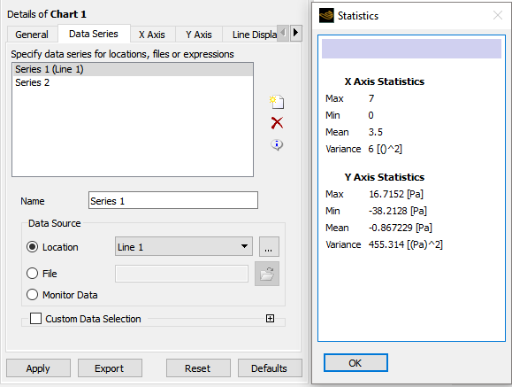
The fields in the Data Source area become enabled after you create an initial series.
For a General > XY chart or a General > Histogram chart, choose a Location or File or Monitor Data to define the source of the data for the series you are creating. A typical location would be a line or a streamline; a typical data file would be a CSV file.
For a General > XY - Transient or Sequence chart, a typical Location would be a point. However, such a chart will also accept a File or Expression or Monitor Data as the data source. For example, you could use an expression to plot
areaAve(Temperature)@Outletas a function of time.
The data delimiter in a data source file is usually a comma.[4]
Files that use commas as delimiters have at least one section
of numerical data. If there is only one section of data, then the
name specification (consisting of the [Name] header
and the line that follows it) and the [Data] header
are optional, but not independently; they must either be both included
or both omitted. If there is more than one section of data, the name
specification and [Data] header are both required.
The line that follows the [Data] header is always
optional; omitting it causes default variable names and default units
to be assumed. An example section follows:
[Name]
Velocity Profile

[Data]
 Z [ m ],Velocity [ m s^-1 ]
-0.10000000,4.53693390
-0.09797980,4.54303789
-0.09595960,4.54667473
-0.09393939,4.54347515
-0.09191919,4.54762697
...
The line following the keyword [Data] may specify the variable names and units for each column of numerical
data that follows. If variable names are not provided, default names
are applied.
This is the same format as the export file in CFD-Post. It is also the same format that CFX-Solver Manager uses when exporting lines from a chart. Data exported from these sources can be imported directly into CFD-Post to produce a chart line.
For Histograms, the second column is used as the variable data.
Note: When exporting histogram data, the Y Axis data (that is, the counts) will be stored in the CSV file with the variable name "Count(Histogram Data)". The "(Histogram Data)" suffix is required if this information is imported into CFD-Post because it indicates to CFD-Post that this variable must be interpreted as histogram data and not as regular chart line data.
Note: If File is selected as the data source for a Transient or Sequence chart, and a Fast Fourier Transform (FFT) is being calculated, then the data in the file must be in particular units:
If the FFT X Function setting has a value of
Strouhal Number,Octave Band FullorOne Third Full, the X Axis data in the file must have units of[s](seconds).If the FFT Y Function setting has a value of
Sound Amplitude,Sound Pressure Level,A Weighted,B WeightedorC Weighted, then the Y Axis data in the file must have units of[Pa](Pascals).
The File Variable Selection settings are available when you are defining a data series from a file. They indicate which data, within the selected file, is to be used to define the data series.
Section Name is used to select a section of data from the file. This setting does not appear if there is only one section of data in the data source file.
X Axis Variable and Y Axis Variable specify which two columns of data are to be used to generate a chart line.
The Custom Data Selection Controls settings are available when you are defining a data series from a location or expression, with General > Fast Fourier Transform not selected.
When selected, the Custom Data Selection controls enable you to override the settings on the X Axis and Y Axis tabs for each series individually. See Chart: X Axis Tab and Chart: Y Axis Tab for more details on what each setting means.
You can also specify the use of Hybrid or Conservative values or to use the absolute value of data points. For help on the use of Hybrid or Conservative values, see Hybrid and Conservative Variable Values.
Other available settings depend on the chart type; see X Axis Data Selection for details.
The Monitor Variable Selection settings are available when you are defining a data series from monitor data or solution residuals.
Set Source to one of:
Current Cases
Monitor data from all cases are included in the series, as separate lines. For example, if results files StaticMixer_001.res and StaticMixerRef_001.res are loaded and the residual monitor
MAX P-Massis selected for the series, then multiple lines will be generated, one for each results file.File
Monitor data is taken from the file you specify. The allowed file types are .res, .mres, .bak, and .mon.
X Axis Variable and Y Axis Variable specify which variables are to be used to generate a chart line.
Take absolute value of data points controls whether the values of data points are always positive.
Note: If a complete multi-configuration (.mres) run is loaded as a single case, only the monitor data that is present in the last configuration will be added to the series.
The X Axis tab is used to set properties for all data series that do not have custom data selection (which is set on the Series tab). The options available on the X Axis tab vary according to the General tab's Type setting.
The Data Selection settings control which variable is used as the data source and how the data is processed:
When General > Type is XY or Histogram, the Variable field can be set to any variable. Hybrid vs. Conservative sets how conservation equations
for the boundary control volumes are solved. See Hybrid and Conservative Variable Values for details. Take absolute value of data points controls whether the
values of data points are always positive.
When General > Type is XY — Transient or Sequence, the Expression field can be set to expressions provided in CFD-Post or
to expressions that you have defined. For example, you could use this
option to plot areaAve(Temperature)@Outlet as a function of time.
When General > Type is XY — Transient or Sequence and Fast Fourier Transform is selected, you can define an X Function.
The options for the X Function are related to the discrete frequencies
at which the Fourier coefficients are computed. You can apply the
following specific analytic functions. Because the corresponding definitions
for the y-axis functions include contributions from both elements
of a complex conjugate pair (i.e.  and
and  ), definitions are
provided for
), definitions are
provided for  when
when  is even, and
  when
when  is odd.
is defined as:
 | (12–51) |
where N is the number of data points used in the FFT.
is the nondimensionalized version of the frequency defined in the equation for :
 | (12–52) |
where  and
and  are the reference length and velocity scales. Note
that you can set
are the reference length and velocity scales. Note
that you can set  and
and  by clicking on the General tab.
Fourier Mode is the index in
 | (12–53) |
and/or
 | (12–54) |
which represents the nth or kth term in the Fourier transform of the signal.
Octave Band Full is a range of discrete frequency bands for different octaves within the threshold of hearing. The range of each octave band is double to that of the previous band (see Table 12.3: Octave Band Frequencies and Weightings).
One Third Full is a range of discrete frequency bands within the threshold of hearing. Here the range of each band is one-third of an octave, meaning that there are three times as many bands for the same frequency range.
Table 12.3: Octave Band Frequencies and Weightings
| Lower Freq. (Hz) | Center Freq. (Hz) | Upper Freq. (Hz) | dB A | dB B | dB C |
|---|---|---|---|---|---|
| 11 | 16 | 22 | -56.7 | –28.5 | -8.5 |
| 22 | 31.5 | 45 | -39.4 | -17.1 | -3.0 |
| 45 | 63 | 90 | -26.2 | -9.3 | -0.8 |
| 90 | 125 | 180 | -16.1 | -4.2 | -0.2 |
| 180 | 250 | 355 | -8.6 | -1.3 | 0.0 |
| 355 | 500 | 710 | -3.2 | -0.3 | 0.0 |
| 710 | 1000 | 1400 | 0.0 | 0.0 | 0.0 |
| 1400 | 2000 | 2800 | 1.2 | -0.1 | -0.2 |
| 2800 | 4000 | 5600 | 1.0 | -0.7 | -0.8 |
| 5600 | 8000 | 11200 | -1.1 | -2.9 | -3.0 |
| 11200 | 16000 | 22400 | -6.6 | -8.4 | -8.5 |
These controls are enabled when the chart type is Histogram.
If Category Divisions are set to Automatic, you are able to specify the Number of Divisions. If Category Divisions are set to User Defined, you are able to specify the Division Values.
The Division Values field enables you to
type points where you want to create histogram boundaries. You can
either enter user-defined category divisions by typing a comma-separated
ordered list directly into the Division Values field, or click More  to open up an editor for the division values
(which includes the ability to set the values in a particular unit).
If you use the editor, then the values do not need to be entered in
order as you will be offered the chance to sort the values when you
close the editor.
to open up an editor for the division values
(which includes the ability to set the values in a particular unit).
If you use the editor, then the values do not need to be entered in
order as you will be offered the chance to sort the values when you
close the editor.
You can choose to Determine ranges automatically or to set Min and Max values.
To get the range for the Min and Max values, click Get range from existing chart .
The default X-axis scale is linear but can be set to be a Logarithmic scale. Select Invert Axis to reverse the direction of the scale.
You can have axis numbers set automatically or choose the format yourself:
If you select Determine the number formatting automatically, CFD-Post will change the formatting to the one that best suits the data being plotted.
If you clear Determine the number formatting automatically, you can choose between scientific notation and fixed notation, and set the amount of precision.
The Y Axis tab is used to define the characteristics of the Y axis of the chart you are going to produce. For descriptions of many of the fields on this tab, see Chart: X Axis Tab. Fields unique to this tab are described below.
When the General tab is set to create an
XY or an XY transient or sequence chart, the Data Selection includes a Variable that you can set; you can
also control whether the boundary data is Hybrid or Conservative, and whether or not to take
the absolute value of data points.
When the General tab is set to create a histogram, the Y axis Value can be:
CountWhen
Countis selected, the display shows the number of values lying within each category, or, if the Weighting is not set toNone, the total weight within the category.PercentageWhen
Percentageis selected, the display is scaled to show the percentage of values or weights lying within each category. ThePercentageis calculated using all of the data on the selected location, even if some of the data is not displayed because it lies outside of the selected category boundaries. Hence the totalPercentageshown in the selected categories may add up to less than 100%.
The Weighting can be:
NoneGeometricalMass Flow
The weighting setting changes the shape of the histogram
by removing mesh dependencies. For example, if mesh density varies
along a line, counts are biased towards areas of higher density; the Geometrical setting removes that bias.
When the General tab is set to Fast Fourier Transform, a Y Function field appears where you can choose one of the following settings.
The definitions are provided for  when
when  is even, and
  when
when  is odd. The definitions include contributions from
both elements of a complex conjugate pair:
is odd. The definitions include contributions from
both elements of a complex conjugate pair:  and
and  .
.
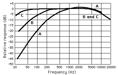
- A Weighted, Sound Pressure Level (dB A)
This is the calculated sound pressure level weighted by the A-scale function to more closely approximate the frequency response of the human ear. A-weighting is applied for loudness levels below 55 phons (55 dB at 1 kHz) and is the most commonly used weighting function. See Figure 12.2: A-, B-, and C-weighting Functions for a graphical representation. This option is available only when X Function on the X-Axis tab is set to
Octave Band FullorOne Third Full.- B Weighted, Sound Pressure Level (dB B)
This is the calculated sound pressure level weighted by the B-scale function. B-weighting is applied for loudness levels between 55 and 85 phons, though it is rarely used. See Figure 12.2: A-, B-, and C-weighting Functions for a graphical representation. This option is available only when X Function on the X-Axis tab is set to
Octave Band FullorOne Third Full.- C Weighted, Sound Pressure Level (dB C)
This is the calculated sound pressure level weighted by the C-scale function. C-weighting is applied for loudness levels above 85 phons and is commonly used for high-intensity sounds such as traffic studies. See Figure 12.2: A-, B-, and C-weighting Functions for a graphical representation. This option is available only when X Function on the X-Axis tab is set to
Octave Band FullorOne Third Full.
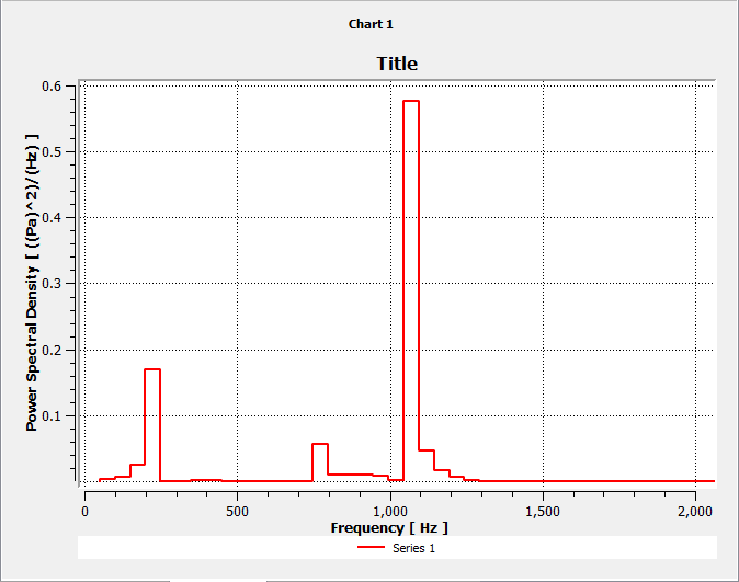
- Power Spectral Density
This is the distribution of signal power in the frequency domain. Its value and units depend on the choice of X Function. For the detailed spectral representation with all resolved harmonics (that is, when the X Function option is set to either
Frequency,Strouhal Number, orFourier Mode), the power spectral density ( ) has
units of the signal magnitude squared over the frequency (for example,
Pa2/Hz) and is defined for the frequency
) has
units of the signal magnitude squared over the frequency (for example,
Pa2/Hz) and is defined for the frequency  as
as
(12–55)
where
 is the frequency
step in the discrete spectrum, and
is the frequency
step in the discrete spectrum, and  is the Fourier
mode power.
is the Fourier
mode power. When
 is even, the Fourier mode power is computed as:
(12–56)
When
 is odd, the Fourier mode power is computed as:
(12–57)
For the octave analysis (that is, when the X Function option is set to either
Octave Band FullorOne Third Full), the power spectral density has units of the signal magnitude squared (for example, Pa2), and is defined for the frequency band as
as 
(12–58)
where
 includes all of the Fourier modes belonging to the
band.
includes all of the Fourier modes belonging to the
band.- Sound Amplitude
This is similar to the
Sound Pressure Level (dB)option, and is a logarithmic conversion of the pressure signalMagnitudeinto decibel units. The sound amplitude in dB, , is calculated for either a Fourier mode
or a frequency band using
, is calculated for either a Fourier mode
or a frequency band using
(12–59)
- Sound Pressure Level
This is the decibel level. For either general or acoustic data, when the sampled data is pressure (for example, static pressure or sound pressure), the sound pressure level in dB,
 , is calculated in decibel
units using
, is calculated in decibel
units using 
(12–60)
where
 is
the power spectral density for either a particular Fourier mode or
a particular frequency band (see Equation 12–55 and Equation 12–58).
is
the power spectral density for either a particular Fourier mode or
a particular frequency band (see Equation 12–55 and Equation 12–58).  is the reference acoustic pressure, with
a default value of
is the reference acoustic pressure, with
a default value of  Pa.
Pa.- Magnitude
This is the amplitude. For the detailed spectral representation with all resolved harmonics (that is, when the X Function option is set to either
Frequency,Strouhal Number, orFourier Mode), the magnitude ( ) is defined for the frequency
  in one of two ways.
When
 is even:
(12–61)
When
 is odd:
(12–62)
where, in both cases,
 is the mean signal value.
For the octave analysis (that is, when the X Axis Function is either
Octave Bandor1/3-Octave Band), the magnitude is defined for the frequency band as
as 
(12–63)
where
 is calculated according to Equation 12–58.
On the Line Display tab you can set the Line Style to a variety of settings, including Automatic, Solid, Dash, Dot, and so on.
For scatter charts, Automatic is interpreted as
None, although you can add lines to scatter charts if desired. Note that
If lines are manually added to a scatter chart, the points are joined in the order that
CFD-Post reads them and do not represent any underlying data structures.
You can select the Use series name for legend name check box to derive the name of the line (as it appears in the legend) from the name of the series (as defined on the Data Series tab and, if more than one case is loaded, from the case name). Alternatively, you can clear that check box and type in a new Legend Name.
You can have CFD-Post Automatically generate Line Color or you can:
Clear the Automatically generate Line Color check box.
Optionally click the bar beside Line Color to cycle through 10 basic colors. Click the right-mouse button to cycle backwards. Alternatively, you can choose any color by clicking Color selector
to the right of the Line
Color setting.Optionally change the selection for Line Type or FFT Line Type. For details, see Line Type and FFT Line Type Options.
Use the Symbols drop-down menu to place a graphic at every data point of
the series. Automatic is interpreted as None for
line charts and, for scatter charts, chooses a different symbol for each data set.
Use the Symbol Color control to set a color for the graphic the same way you did for the Line Color or select Automatically generate Symbol Color.
Note: Line width and symbol size can be set on the Chart Display tab for the chart as a whole, but cannot be set for each line individually.
On the General tab, if Fast Fourier Transform is selected, the line type is controlled by the FFT Line Type setting, otherwise, the line type is controlled by the Line Type setting; the applicable setting is shown.
Both the FFT Line Type and Line Type settings have the following options:
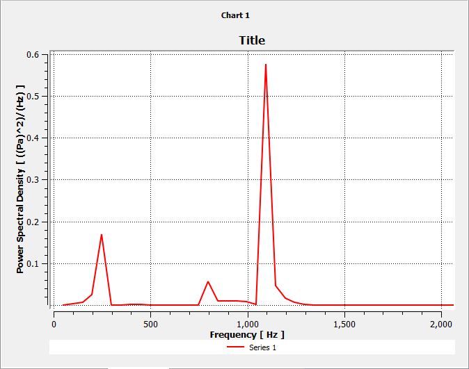
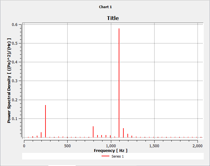
Lines(the default for non-FFT plots) - This line type is suitable for general plots.Bars(the default for FFT plots) - This line type is suitable for FFT plots.Steps- This line type is suitable for FFT plots.
When Fill Area is selected, you can choose
to have a fill color generated automatically or at all times (Always On). The Automatic setting
generates a fill when the chart's General tab's Type is set to Histogram.
Note: Plotting fill areas for graphs that have multiple y values for a given x (such as streamlines) does not produce useful results.
The following sections describe the Chart Display tab.
The legend is the text that you entered in the Name field on the Data Series tab displayed beside the line color that represents its data source.
When Display Legend is selected, the chart's legend appears, either Outside Chart or Inside Chart.
When Outside Chart is selected, set the Location and Justification of the legend:
Location is
BeloworAbove, Justification can beLeft,Center, orRight.Location is
RightorLeft, Justification can beTop,Center, orBottom.
When Inside Chart is selected, the legend is displayed in a box that appears on the chart. Use the X Justification and Y Justification controls to locate a fixed-size box at standard locations, optionally using Width/Height to change the size of the box. Alternatively, set X Justification and Y Justification to None so that you can use Position and Width/Height to control the size and position of the box exactly.
Here you set the width of the line and the size of the symbol (if any) that you defined on the Line Display tab. These sizes apply to all lines and all symbols (you cannot set sizes for individual lines or symbols).
Here is where you control the font type and size of the Title (which you defined on the General tab), the Axes Titles, the Axes values, and the Legend.
Note: By default, the titles of the axes are derived from the variables used in the line definition (not necessarily from the X Axis and Y Axis tabs because a transient chart that uses an expression and any chart that uses custom data selection will set the variables used directly). You can override these default titles by going to the X Axis and Y Axis tabs, clearing the Use data for axis labels check box, and typing in a Custom Label name.
The legend text is defined by default as a combination of the series definitions on the Series tab and, when more than one case is loaded, the case names, but can be specified on a line-by-line basis directly on the Line Display tab by clearing the Use series name for legend name check box and typing in a Legend Name.
[4] There are two exceptions to this: if the extension of the file is .xy, then the delimiter is a tab character; If the extension of the file is .out, then the delimiter is a space character.