


When the dynamics of a cable are included in the cable motion analysis, the effects of the cable mass, drag forces, inline elastic tension, and bending moment are considered. Forces on the cable will vary in time, and the cable will generally respond in a nonlinear manner. The solution is fully coupled: the cable tensions and motions of the vessel are considered to be mutually interactive, where cables affect vessel motion and vice versa.
The simulation of cable dynamics in Aqwa uses a discretization along the cable length and an assembly of the mass and applied/internal forces. In principle, this approach should give the same solution as any of the methods applied in Aqwa that have been described previously. However, in the case of a dynamic cable the inline stiffness is extremely large compared with the transverse stiffness. In addition, the sea bed is modeled with nonlinear springs and dampers, chosen to minimize discontinuities and energy losses at the touchdown point due to the discretization. Forces on each element of the cable are determined and assembled into a symmetric banded global system ready for solution directly (in the static/frequency domain) or by integrating in time.
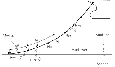
Figure 9.8: Modeling of a Dynamic Cable shows the configuration of a dynamic cable in discrete form in
the fixed reference axes (FRA). Each dynamic mooring line is modeled
as a chain of Morison-type elements subjected to various external
forces.  denotes
the unit axial vector from the j-th node to the (j+1)-th node
in the fixed reference axes, while
denotes
the unit axial vector from the j-th node to the (j+1)-th node
in the fixed reference axes, while  is the unstretched cable length from the anchor
point (or the first attachment point on the structure) to the j-th node. The sea bed is assumed to be horizontal
and flat. The reaction force of the sea bed on the mooring line is
modeled by mud line springs at each node. Each mud line spring is
attached between the top of the artificial mud layer and the cable
element node, if the node is located below the mud line level. The
depth of the mud layer is
is the unstretched cable length from the anchor
point (or the first attachment point on the structure) to the j-th node. The sea bed is assumed to be horizontal
and flat. The reaction force of the sea bed on the mooring line is
modeled by mud line springs at each node. Each mud line spring is
attached between the top of the artificial mud layer and the cable
element node, if the node is located below the mud line level. The
depth of the mud layer is  above
the seabed. The laid length
above
the seabed. The laid length  of a dynamic mooring line on the sea bed is measured from the anchor
to the touchdown point, which is defined as
of a dynamic mooring line on the sea bed is measured from the anchor
to the touchdown point, which is defined as  above the seabed.
A single element of a circular slender cable is shown in Figure 9.9: Forces on a Cable Element, which is subjected to external hydrodynamic loadings as well as to structural inertia loading. Torsional deformation is not included in Aqwa dynamic cable analysis.
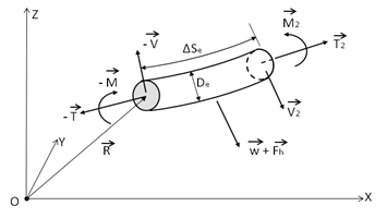
The motion equation of this cable element is
 | (9–45) |
where  is the structural mass per unit
length,
is the structural mass per unit
length,  is the distributed moment loading per unit length,
  is the position vector of the first node
of the cable element,
is the position vector of the first node
of the cable element,  and
and  are the length and diameter of the element respectively,
  and
and  are the element weight
and external hydrodynamic loading vectors per unit length respectively,
are the element weight
and external hydrodynamic loading vectors per unit length respectively,  is the tension force vector at the first
node of the element,
is the tension force vector at the first
node of the element,  is the bending moment vector at the first node of the element, and
  is the shear force vector at the first
node of the element.
is the shear force vector at the first
node of the element.
The bending moment and tension are related
to the bending stiffness  and the axial stiffness
  of the cable material through the following relations:
 | (9–46) |
where  is the axial strain of the element.
To ensure a unique solution to Equation 9–45, pinned connection boundary conditions are imposed at the top and bottom ends:
 | (9–47) |
where  are the locations of
the cable attachment points and
are the locations of
the cable attachment points and  is the total unstretched length of the cable.
The dynamic response of the cable with bending governed by Equation 9–45, Equation 9–46, and Equation 9–47 is solved numerically by employing the discrete Lump-Mass model. As shown in Figure 9.8: Modeling of a Dynamic Cable, the cable is discretized into a number of finite elements where the mass of each element is concentrated into a corresponding node.
The unit axial vector  of an element j, which corresponds
to the slope of that element, from one element to the next, is given
by:
of an element j, which corresponds
to the slope of that element, from one element to the next, is given
by:
 | (9–48) |
where the unstretched element length is  .
.
The curvature vector at node j is given by the rate of change of slope, which can be calculated from the cross product of the unit vectors along two adjacent elements, i.e.
 | (9–49) |
where the effective length of the j-th node in this context is  .
.
 is assumed to be
constant between two adjacent elements. From Equation 9–46 the bending moment at node j is:
is assumed to be
constant between two adjacent elements. From Equation 9–46 the bending moment at node j is:
 | (9–50) |
For the general configuration of cables,
the axial stiffness  is of a higher order
than the bending stiffness
is of a higher order
than the bending stiffness  , so that we may
assume that the axial strain is small and the bending stiffness factor
, so that we may
assume that the axial strain is small and the bending stiffness factor  is constant.
The 3×3 axial and normal directional tensors are now introduced, as
 | (9–51) |
If the distributed bending moment is zero, from Equation 9–45 and Equation 9–51 the matrix form of the shear force on element j is expressed as
 | (9–52) |
Integrating both sides of the motion equation given in Equation 9–45, for an element j, the motion of that element with respect to its two ends can be expressed in a matrix form:
 | (9–53) |
in which  is the
shear force at node j, which is
calculated from the two adjacent elements. Note that in the current
notation, an index in parentheses e.g. (j) refers to an element, while an index without the parentheses refers
to a node.
is the
shear force at node j, which is
calculated from the two adjacent elements. Note that in the current
notation, an index in parentheses e.g. (j) refers to an element, while an index without the parentheses refers
to a node.
To maintain generality, assume that there is an intermediate clump weight/buoy attached at node j, but no clump/buoy mass is attached at node j+1. The mass of this clump weight/buoy is M. Then the total gravity forces at node j and node j+1 for the element (j), in a 6×1 matrix form and in the fixed reference axes, are
 | (9–54) |
where  is the acceleration due to gravity. We assume that half of the gravitational
force due to the clump weight/buoy will act on the other (i.e. the adjacent) element to which the
j-th node is attached.
is the acceleration due to gravity. We assume that half of the gravitational
force due to the clump weight/buoy will act on the other (i.e. the adjacent) element to which the
j-th node is attached.
The wave excitation force on a dynamic
cable is ignored. Hence in Equation 9–53 the hydrodynamic force,  , acting on a cable element consists of the buoyant
force, the drag force, and the (added mass related) radiation force,
for example
, acting on a cable element consists of the buoyant
force, the drag force, and the (added mass related) radiation force,
for example
 | (9–55) |
where  is the cable element added mass matrix including the added mass contribution of
the attached intermediate clump weight/buoy, and
is the cable element added mass matrix including the added mass contribution of
the attached intermediate clump weight/buoy, and  is the acceleration of the cable at node j.
Denoting the equivalent cross-sectional area of the mooring line as
 and the displaced mass of water of the intermediate clump weight/buoy as
 , the element buoyant force matrix is
 | (9–56) |
where  is the density of water.
The time-dependent drag force on the mooring line element is expressed in a simplified form as
 | (9–57) |
where  is the matrix form of the structural velocity at node j at time t,
  is the matrix form of the current velocity at the location of node j ,
  is the drag coefficient of the clump weight/buoy (attached at node j) which has corresponding projected surface area
  , and the drag force on node j connected to a mooring line
element is
, and the drag force on node j connected to a mooring line
element is

in which  and
and  are the transverse and inline drag coefficients respectively.
Equation 9–57 provides a simplified form of the drag force on a mooring line element; a more accurate form may be applied by integrating the drag force over the length of the element to take the variation of the current velocity along the element into account. This is performed in Aqwa using a Gaussian integration scheme.
The reaction force of the sea bed on
the mooring line is modeled by a mud line spring at each node within
the mud layer. If the position of node j is  , the water depth is
  , and the depth of the mud layer
is
, and the depth of the mud layer
is  ,
the magnitude of the reaction force due to the mud spring on node j is defined as
,
the magnitude of the reaction force due to the mud spring on node j is defined as
 | (9–58) |
where  is the net mass at node j, i.e.
 = structural mass - displaced mass of water, and
  .
.
It is also assumed that the mud line springs are critically damped, where the damping force at node j in the vertical direction is defined as
 | (9–59) |
where  is the sum of the structural
mass and added mass at node j.
is the sum of the structural
mass and added mass at node j.
The Coulomb friction model is applied for the estimation of sea bed friction force on dynamic cables. The Coulomb function is written as:
 | (9–60) |
where  is the constant friction coefficient, and
  is the magnitude of the normal reaction force of the sea bed.
The direction of the friction force is opposite to the in-plane velocity of the cable on the sea bed, so Equation 9–60 could be rewritten as
 | (9–61) |
where  is the in-plane velocity of the laid-down segment of a mooring line on the sea
bed and
is the in-plane velocity of the laid-down segment of a mooring line on the sea
bed and  .
.
To avoid numerical instability problems when the slip velocity or the movement changes direction, the friction force is set to be linear or nonlinear varying within a transition zone [35]. By introducing a single parameter transition function, the extended Coulomb friction model is expressed as:
 | (9–62) |
where  is the ramp velocity threshold (or critical velocity),
  is the transition function, which satisfies
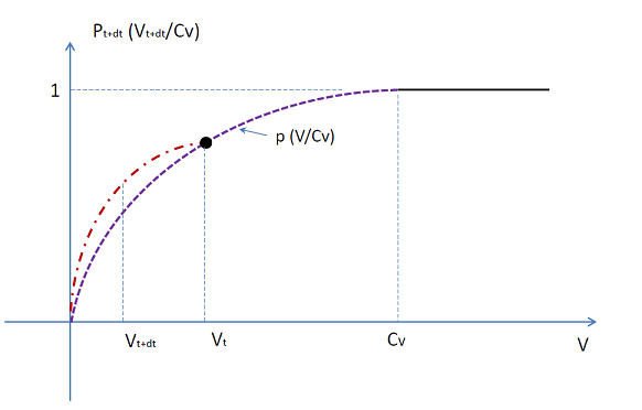
  , as shown in Figure 9.10: Double Quadratic Transition Function.
In the Aqwa time domain dynamic cable analysis, the ramp velocity threshold is defined as:
 | (9–63) |
where  is the diameter of the cable and
  is the zero-cross or characteristic wave period.
A second-order polynomial form of the transition function is introduced
by Ostergaard et. al. [35], which is determined with an additional
condition of  when
when  :
:
 | (9–64) |
A double quadratic extension Coulomb friction mode, as shown in Figure 9.10: Double Quadratic Transition Function, is introduced in Aqwa time domain analysis to smooth the variation of friction when the magnitude of node velocity decreases compared to the previous time step.
The double quadratic transition function in Aqwa time domain analysis is expressed as:
 | (9–65) |
In Equation 9–65, the single parameter
transition function  is given by Equation 9–64.
If the axial and lateral friction coefficients  and
and  are different, the equivalent friction coefficient is defined as:
 | (9–66) |
where  and
and  are the cable velocity components in the sea bed inline and lateral directions,
respectively.
are the cable velocity components in the sea bed inline and lateral directions,
respectively.
It is found from Equation 9–66 that  if
if  .
.
It is assumed that the friction force may exist once a cable segment node (node j) touches down:
 | (9–67) |
where  is the water depth at the j-th node location
and
is the water depth at the j-th node location
and  is the depth of the mud layer shown in Figure 9.8: Modeling of a Dynamic Cable.
The element bending stiffness matrix can be determined directly from the derivative of the shear force:
 | (9–68) |
From Equation 9–52, it can be seen that the shear force on element j is a function of the positions of four
nodes, j-1, j, j+1, and j+2 (for the evaluation of  and
and  , defined by Equation 9–48) so that
  is a 12×12 matrix. Denoting
the movements at these four nodes as [u
j-1], [u
j], [u
j+1], [u
j+2] and substituting Equation 9–52 into Equation 9–68, we have
is a 12×12 matrix. Denoting
the movements at these four nodes as [u
j-1], [u
j], [u
j+1], [u
j+2] and substituting Equation 9–52 into Equation 9–68, we have
 | (9–69) |
where
 | (9–70) |
in which  is the gradient operator with
respect to the displacement at node
is the gradient operator with
respect to the displacement at node  and
and

The axial elastic force on element (j) is a function of the deformations of two nodes, i.e. [u j], [u j+1],
 | (9–71) |
where  is the 6×6 stiffness matrix of the mooring
line element:
is the 6×6 stiffness matrix of the mooring
line element:
 | (9–72) |
In which  is the inline linear stiffness or the equivalent
inline stiffness for a nonlinear axial stiffness cable, which is discussed
in Catenary Segment with Influence of Axial Nonlinear Elasticity.
is the inline linear stiffness or the equivalent
inline stiffness for a nonlinear axial stiffness cable, which is discussed
in Catenary Segment with Influence of Axial Nonlinear Elasticity.
Assembling the matrices of all the elements and applying boundary conditions on the two attachment points of the mooring line, the static solution can be solved by
 | (9–73) |
where  is the assembled total static
force matrix.
is the assembled total static
force matrix.
In a time domain analysis, the solution of dynamic cable motion at the given attachment locations can be obtained by solving the following equation
 | (9–74) |
where  and
and  are the assembled
total force matrix and the total mass matrix (including structural
and added masses) respectively.
are the assembled
total force matrix and the total mass matrix (including structural
and added masses) respectively.
In a frequency domain analysis, all of the nonlinear terms are linearized such that
 | (9–75) |
where  is the linearized damping matrix.
In Equation 9–75, the linearized damping is obtained from the root mean square of the relative velocity for multiple frequency solutions. The numerical approach is similar to the Morison drag linearization discussed in Morison Drag Linearization.
In summary, the forces applied on the dynamic cable in the different analysis procedures are listed in Table 9.1: Summary of Force Components on Dynamic Cable.
Table 9.1: Summary of Force Components on Dynamic Cable
| Forces applied | Equilibrium | Frequency domain | Time domain |
|---|---|---|---|
| Gravitational force (cable and clump weight/buoy) | √ | - | √ |
| Buoyant force (cable and clump weight/buoy) | √ | - | √ |
| Structural inertia force (cable and clump weight/buoy) | - | √ | √ |
| Radiation force due to added mass | - | √ | √ |
| Drag force due to current and/or cable motion | √ | Linearized | √ |
| Linear or nonlinear axial tension | √ | Linearized | √ |
| Bending moment due to cable bending stiffness | √ | √ | √ |
| Seabed effect by mud-layer spring stiffness | √ | Linearized | √ |
| Seabed effect by mud-layer spring damping | - | Linearized | √ |
| Seabed friction | - | - | √ |
| Wave excitation force on cable | - | - | - |
| Torsional moment | - | - | - |
| Reaction forces at two ends | √ | √ | √ |
Note: The check mark ' √ ' indicates the item is included, ' - ' indicates the item is excluded.