1.3. Demonstration Problem 1

Problem Description

A cantilevered bend pipe is modeled with a ratio of outer radius to wall thickness equal to 45.36. Single point response spectrum analysis is performed on the model with base excitation along the global X, Y and Z directions.

The input files for this problem are listed below:

demonstration-problem1-290 Input Listing

demonstration-problem1-281 Input Listing

demonstration-problem1-18 Input Listing

Material Properties:

Young's modulus = 24e6 psi

Poisson's ratio = 0.3

Density = 0.000125 lb-sec²/in⁴

Geometric Properties:

Outer diameter = 10.932 inches

Wall thickness = 0.1205 inches

Radius of curvature = 36.30 inches

Loading:

Acceleration response spectrum curve is input on the SV and FREQ commands.

Results

Figure 1.1: Nodal Equivalent Stress Plot Obtained from PIPE18 Elements

Figure 1.2: Nodal Equivalent Stress Plot Obtained from ELBOW290 Elements

Figure 1.3: Nodal Equivalent Stress Plot Obtained from SHELL281 Elements

Results Comparison

Table 1.1: Frequencies Obtained from Modal Solution

Mode	Results from SHELL281 (A)	Results from PIPE18 (B)	Results from ELBOW290 (C)	Ratio between A and B	Ratio between A and C
1	145.554	90.588	145.641	1.606	0.999
2	149.530	100.503	149.613	1.487	0.999
3	315.404	418.040	315.392	0.754	1.000
4	319.433	480.193	319.425	0.665	1.000
5	575.655	1241.493	575.845	0.463	0.999
6	604.193	1335.526	604.387	0.452	0.999
7	757.127	2260.454	757.039	0.334	1.000
8	760.925	2505.754	760.827	0.303	1.000
9	947.803	2771.559	948.182	0.341	0.999
10	982.926	3852.258	983.168	0.255	0.999
11	1001.878	3852.333	1001.868	0.260	1.000
12	1242.305	5223.342	1242.931	0.237	0.999
13	1271.296	5279.894	1271.867	0.240	0.999
14	1368.966	6010.645	1368.740	0.227	1.000
15	1411.341	6673.827	1411.654	0.211	0.999

Table 1.2: Displacements and Stresses Obtained from Spectrum Solution

Result Quantities	Results from SHELL281 (A)	Results from PIPE18 (B)	Results from ELBOW290 (C)	Ratio between A and B	Ratio between A and C
Maximum displacement Vector Sum	4.99 x 10^-4	1.23 x 10^-3	4.94 x 10^-4	0.407	1.012
Maximum equivalent stress	33.144	41.915	27.633	0.790	1.199

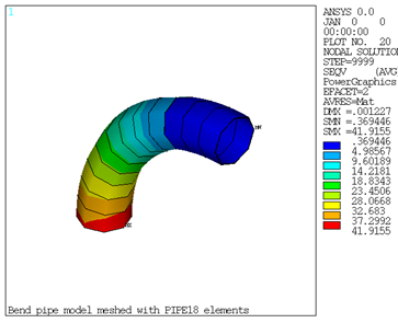
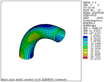
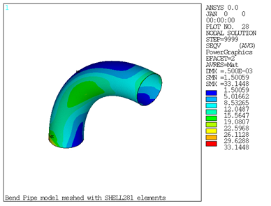
Conclusion

The result comparison table and Figure 1.1: Nodal Equivalent Stress Plot Obtained from PIPE18 Elements, Figure 1.2: Nodal Equivalent Stress Plot Obtained from ELBOW290 Elements, and Figure 1.3: Nodal Equivalent Stress Plot Obtained from SHELL281 Elements show that the results obtained from modal and spectrum analyses with ELBOW290 elements closely match with the results obtained from SHELL281 elements. The results obtained from PIPE18 elements are off by more than 50% when compared with SHELL281 results due to the limitations explained in Piping Benchmarks using Current Technology Elements.