


VM-NR1677-01-7-a
VM-NR1677-01-7-a
NUREG/CR-1677: Volume 1, Benchmark Problem No. 7
Overview
Test Case
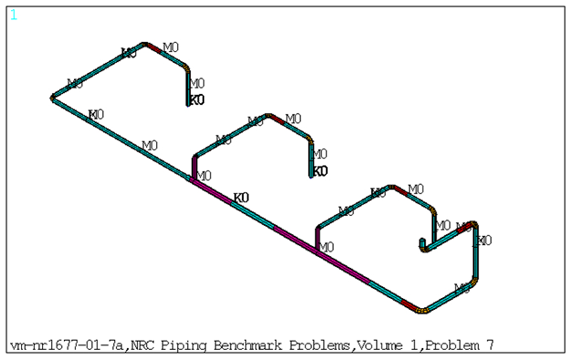
This benchmark problem is a multi-branched configuration containing four anchor points. The problem represents an actual piping system as shown in Figure 625: FE Model of the Benchmark Problem. Modal and response spectrum analysis is performed on the piping model. The input excitation consists of two distinct sets of excitation spectra. Frequencies obtained from modal solve and the nodal/element solution obtained from spectrum solve are compared against reference results.
| Material Properties | Geometric Properties | Loading | |||||||||||||||||||||||||||||||||||||||
|---|---|---|---|---|---|---|---|---|---|---|---|---|---|---|---|---|---|---|---|---|---|---|---|---|---|---|---|---|---|---|---|---|---|---|---|---|---|---|---|---|---|
Pipe Elements: Material ID 1:
Material ID 2:
Stiffness for Spring –Damper Elements (lb/in): Since there are multiple Spring Supports at different locations, the Stiffness for the Spring Damper Elements are listed based on real constant set number. Set 1:
Set 23:
Set 24:
Mass Elements (lb-sec2/in): (Isotropic Mass) Set 6:
Set 7:
Set 8:
Set 9:
Set 10:
Set 11:
Set 12:
Set 13:
Set 14:
Set 15:
Set 16:
Set 17:
Set 18:
Set 19:
Set 20:
Set 21:
Set 22:
| Straight Pipe: Set 2:
Set 4:
Bend Pipe: Set 3:
Set 5:
| Acceleration response spectrum curve defined by SV and FREQ commands. |
Results Comparison
Table 52: Frequencies Obtained from Modal Solution
| Mode | Target | Mechanical APDL | Ratio |
|---|---|---|---|
| 1 | 5.034 | 5.033 | 1.000 |
| 2 | 7.813 | 7.812 | 1.000 |
| 3 | 8.193 | 8.192 | 1.000 |
| 4 | 8.977 | 8.977 | 1.000 |
| 5 | 9.312 | 9.312 | 1.000 |
| 6 | 9.895 | 9.895 | 1.000 |
| 7 | 13.220 | 13.221 | 1.000 |
| 8 | 14.960 | 14.956 | 1.000 |
| 9 | 15.070 | 15.066 | 1.000 |
| 10 | 17.750 | 17.754 | 1.000 |
| 11 | 18.210 | 18.208 | 1.000 |
| 12 | 22.900 | 22.899 | 1.000 |
| 13 | 25.020 | 25.022 | 1.000 |
| 14 | 25.850 | 25.854 | 1.000 |
| 15 | 26.940 | 26.941 | 1.000 |
| 16 | 28.130 | 28.131 | 1.000 |
| 17 | 30.300 | 30.297 | 1.000 |
| 18 | 35.220 | 35.218 | 1.000 |
| 19 | 37.100 | 37.095 | 1.000 |
| 20 | 42.610 | 42.612 | 1.000 |
| 21 | 44.420 | 44.415 | 1.000 |
| 22 | 48.090 | 48.086 | 1.000 |
Table 53: Maximum Displacements and Rotations Obtained from Spectrum Solve
| Result Node | Target | Mechanical APDL | Ratio |
|---|---|---|---|
| UX at node8 | 0.0847 | 0.0847 | 1.000 |
| UY at node8 | 0.2434 | 0.2434 | 1.000 |
| UZ at node11 | 0.3421 | 0.3421 | 1.000 |
| ROTX at node7 | 0.0058 | 0.0058 | 1.000 |
| ROTY at node14 | 0.0021 | 0.0021 | 1.000 |
| ROTZ at node50 | 0.0012 | 0.0012 | 1.000 |
Table 54: Element Forces and Moments Obtained from Spectrum Solve
| Result | Target | Mechanical APDL | Ratio |
|---|---|---|---|
| Element 1 | |||
| PX(I) | 236.400 | 236.401 | 1.000 |
| VY(I) | 80.7200 | 80.574 | 0.998 |
| VZ(I) | 260.5000 | 266.003 | 1.021 |
| TX(I) | 4947.000 | 4938.015 | 0.998 |
| MY(I) | 22170.000 | 22128.503 | 0.998 |
| MZ(I) | 2106.000 | 2102.161 | 0.998 |
| PX(J) | 236.000 | 236.401 | 1.002 |
| VY(J) | 80.720 | 80.574 | 0.998 |
| VZ(J) | 266.500 | 266.003 | 0.998 |
| TX(J) | 4947.000 | 4938.015 | 0.998 |
| MY(J) | 20590.000 | 20548.191 | 0.998 |
| MZ(J) | 1656.000 | 1653.184 | 0.998 |
| Element 38 | |||
| PX(I) | 50.360 | 50.222 | 0.997 |
| VY(I) | 27.620 | 27.588 | 0.999 |
| VZ(I) | 28.530 | 26.563 | 0.931 |
| TX(I) | 482.000 | 473.398 | 0.982 |
| MY(I) | 96.690 | 92.848 | 0.960 |
| MZ(I) | 1625.000 | 1640.961 | 1.010 |
| PX(J) | 50.360 | 50.222 | 0.997 |
| VY(J) | 27.620 | 27.588 | 0.999 |
| VZ(J) | 28.530 | 26.563 | 0.931 |
| TX(J) | 462.000 | 473.398 | 1.025 |
| MY(J) | 428.000 | 420.239 | 0.982 |
| MZ(J) | 1796.000 | 1790.638 | 0.997 |
| Element 49 | |||
| PX(I) | 94.270 | 92.742 | 0.984 |
| VY(I) | 35.290 | 34.212 | 0.969 |
| VZ(I) | 26.370 | 25.380 | 0.962 |
| TX(I) | 235.400 | 230.264 | 0.978 |
| MY(I) | 2491.000 | 2447.900 | 0.983 |
| MZ(I) | 446.600 | 441.965 | 0.990 |
| PX(J) | 26.070 | 25.380 | 0.974 |
| VY(J) | 35.290 | 34.212 | 0.969 |
| VZ(J) | 94.270 | 92.742 | 0.984 |
| TX(J) | 469.200 | 457.142 | 0.974 |
| MY(J) | 2176.000 | 2133.047 | 0.980 |
| MZ(J) | 134.000 | 136.211 | 1.017 |
Note: PX (I) and PX (J) = Section axial force at node I and J.
VY (I) and VY (J) = Section shear forces along Y direction at node I and J.
VZ (I) and VZ (J) = Section shear forces along Z direction at node I and J.
TX (I) and TX (J) = Section torsional moment at node I and J.
MY (I) and MY (J) = Section bending moments along Y direction at node I and J.
MZ (I) and MZ (J) = Section bending moments along Z direction at node I and J.
The element forces and moments along Y and Z directions are flipped between Mechanical APDL and NRC results.