


VM272
VM272
2D and 3D Frictional Hertz Contact
Overview
| Reference: | Two Dimensional Mortar Contact Methods for Large Deformation Frictional Sliding, International Journal for Numerical Methods in Engineering Vol.62, pp 1183-1225. | ||||||||
| Analysis Type(s): | Static Analysis (ANTYPE = 0) | ||||||||
| Element Type(s): |
| ||||||||
| Input Listing: | vm272.dat |
Test Case
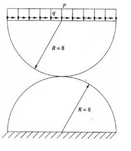
Two parallel linear elastic half cylinders of radius R are pressed by a small distributed pressure p. A tangential pressure, q, is then applied to cause friction at the contact interface. The bottom of the lower cylinder is fixed in all directions. Determine the contact pressure and friction results across the contact interface.
| Material Properties | Geometric Properties | Loading |
E=200.0 N/mm2 v=0.3 | R = 8.0 mm | p=0.625 N/mm q= 0.05851 N/mm |
Analysis Assumptions and Modeling Notes
This problem is solved in two ways:
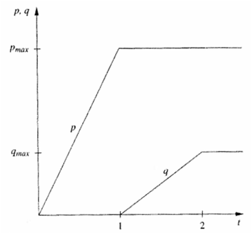
In the first analysis, the cylinders are modeled and meshed with plane elements with plane strain behavior. The problem is solved using 2D surface to surface contact elements with surface-projection definition (KEYOPT(4)=3) and updating contact stiffness based on stresses of underlying elements (KEYOPT(10)=2). In the second analysis, the cylinders are modeled with 3D solid elements with unit thickness in the Z direction. The same element options and contact damping used in 2D analysis are applied to 3D analysis. The simulations use two load steps; the first is a ramped normal pressure of 10 N, applied on the top surface of the upper cylinder, and the second is a ramped tangential pressure of 0.93622 N, also applied to the top surface of the upper cylinder.
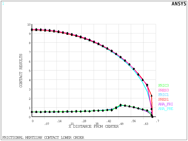
Analytic results approach zero more rapidly than computed results toward the end of the contact interface. These small differences are due to mesh discretization and are considered acceptable.
The plots below show contact pressure and friction with respect to distance along X from the center for both cases.
Results Comparison
Table 14: Contact Pressure 2D
| Location (mm) | Target | Mechanical APDL | Ratio |
|---|---|---|---|
| 0.000 | 9.3514 | 9.3579 | 1.001 |
| 0.100 | 9.2494 | 9.2564 | 1.001 |
| 0.201 | 8.9366 | 8.9485 | 1.001 |
| 0.301 | 8.3896 | 8.4119 | 1.003 |
| 0.401 | 7.5581 | 7.6037 | 1.006 |
| 0.501 | 6.3317 | 6.4303 | 1.016 |
| 0.601 | 4.3924 | 4.6428 | 1.057 |
Table 15: Contact Friction 2D
| Location (mm) | Target | Mechanical APDL | Ratio |
|---|---|---|---|
| 0.000 | 0.5063 | 0.5279 | 1.043 |
| 0.100 | 0.5140 | 0.5302 | 1.032 |
| 0.201 | 0.5395 | 0.5856 | 1.085 |
| 0.301 | 0.5926 | 0.6691 | 1.129 |
| 0.401 | 0.7069 | 0.7877 | 1.114 |
| 0.501 | 1.2663 | 1.2092 | 0.955 |
| 0.601 | 0.8785 | 0.9286 | 1.057 |
Table 16: Contact Pressure 3D
| Location (mm) | Target | Mechanical APDL | Ratio |
|---|---|---|---|
| 0.000 | 9.3514 | 9.4440 | 1.010 |
| 0.100 | 9.2494 | 9.3478 | 1.011 |
| 0.201 | 8.9366 | 9.0350 | 1.011 |
| 0.301 | 8.3896 | 8.4910 | 1.012 |
| 0.401 | 7.5581 | 7.6692 | 1.015 |
| 0.501 | 6.3317 | 6.4495 | 1.019 |
| 0.601 | 4.3924 | 4.5106 | 1.027 |
Table 17: Contact Friction 3D
| Location (mm) | Target | Mechanical APDL | Ratio |
|---|---|---|---|
| 0.000 | 0.5063 | 0.5275 | 1.042 |
| 0.100 | 0.5140 | 0.5428 | 1.056 |
| 0.201 | 0.5395 | 0.5346 | 0.991 |
| 0.301 | 0.5926 | 0.6326 | 1.068 |
| 0.401 | 0.7069 | 0.7553 | 1.068 |
| 0.501 | 1.2663 | 1.2899 | 1.019 |
| 0.601 | 0.8785 | 0.9021 | 1.027 |