


The following topics concerning the analyses results are available:
Prior to solving a harmonic response analysis, it is important to understand the frequency content of the system, and the modal analysis provides this valuable information.
In the solver output, the participation factors in the z (longitudinal) direction are listed at the end of the modal analysis, as follows:
***** PARTICIPATION FACTOR CALCULATION ***** Z DIRECTION
CUMULATIVE RATIO EFF.MASS
MODE FREQUENCY PERIOD PARTIC.FACTOR RATIO EFFECTIVE MASS MASS FRACTION TO TOTAL MASS
1 1947.47 0.51349E-03 0.13955E-03 0.000974 0.194730E-07 0.469851E-06 0.391044E-06
2 1948.16 0.51331E-03 0.39207E-05 0.000027 0.153722E-10 0.470222E-06 0.308693E-09
3 4427.05 0.22588E-03 0.90019E-05 0.000063 0.810341E-10 0.472177E-06 0.162727E-08
4 4427.86 0.22584E-03 -0.46883E-05 0.000033 0.219797E-10 0.472708E-06 0.441383E-09
5 9304.53 0.10747E-03 -0.22162E-05 0.000015 0.491135E-11 0.472826E-06 0.986266E-10
6 9320.90 0.10729E-03 -0.96822E-03 0.006760 0.937453E-06 0.230920E-04 0.188253E-04
7 11382.1 0.87857E-04 0.17053E-05 0.000012 0.290807E-11 0.230921E-04 0.583979E-10
8 11385.3 0.87833E-04 0.53578E-05 0.000037 0.287058E-10 0.230928E-04 0.576451E-09
9 14535.4 0.68797E-04 0.94644E-06 0.000007 0.895743E-12 0.230928E-04 0.179877E-10
10 15206.9 0.65760E-04 -0.14972E-05 0.000010 0.224167E-11 0.230929E-04 0.450157E-10
11 19129.1 0.52276E-04 -0.72228E-04 0.000504 0.521688E-08 0.232187E-04 0.104762E-06
12 19211.2 0.52053E-04 -0.17198E-01 0.120072 0.295763E-03 0.715948E-02 0.593931E-02
13 21192.5 0.47187E-04 -0.13350 0.932096 0.178230E-01 0.437200 0.357911
14 23711.4 0.42174E-04 0.15719E-04 0.000110 0.247096E-09 0.437200 0.496203E-08
15 23712.1 0.42172E-04 0.20055E-03 0.001400 0.402200E-07 0.437201 0.807671E-06
16 26594.1 0.37602E-04 -0.14323 1.000000 0.205145E-01 0.932181 0.411958
17 28705.8 0.34836E-04 0.42418E-05 0.000030 0.179930E-10 0.932181 0.361324E-09
18 29154.9 0.34300E-04 0.10645E-01 0.074323 0.113319E-03 0.934915 0.227559E-02
19 30305.6 0.32997E-04 0.10060E-04 0.000070 0.101211E-09 0.934915 0.203245E-08
20 30312.8 0.32989E-04 0.49382E-04 0.000345 0.243859E-08 0.934915 0.489702E-07
21 34346.4 0.29115E-04 -0.52235E-05 0.000036 0.272853E-10 0.934915 0.547926E-09
22 36793.2 0.27179E-04 0.51304E-02 0.035820 0.263215E-04 0.935550 0.528571E-03
23 44385.1 0.22530E-04 0.22402E-05 0.000016 0.501871E-11 0.935550 0.100782E-09
24 47898.2 0.20878E-04 0.32907E-05 0.000023 0.108290E-10 0.935550 0.217460E-09
25 51110.3 0.19566E-04 -0.82738E-06 0.000006 0.684562E-12 0.935550 0.137469E-10
26 52122.9 0.19185E-04 -0.82532E-06 0.000006 0.681147E-12 0.935550 0.136783E-10
27 52211.6 0.19153E-04 0.43101E-02 0.030092 0.185766E-04 0.935999 0.373043E-03
28 56171.7 0.17803E-04 -0.56272E-05 0.000039 0.316656E-10 0.935999 0.635887E-09
29 56183.0 0.17799E-04 -0.47378E-04 0.000331 0.224465E-08 0.935999 0.450755E-07
30 58861.0 0.16989E-04 0.41097E-01 0.286934 0.168899E-02 0.976751 0.339171E-01
31 60374.9 0.16563E-04 0.41351E-04 0.000289 0.170992E-08 0.976751 0.343375E-07
32 60377.6 0.16562E-04 -0.46874E-04 0.000327 0.219718E-08 0.976751 0.441223E-07
33 62900.6 0.15898E-04 0.58571E-05 0.000041 0.343061E-10 0.976751 0.688912E-09
34 65167.8 0.15345E-04 0.60328E-05 0.000042 0.363949E-10 0.976751 0.730858E-09
35 69986.8 0.14288E-04 0.21853E-02 0.015257 0.477544E-05 0.976866 0.958973E-04
36 72005.0 0.13888E-04 -0.24739E-02 0.017272 0.612022E-05 0.977014 0.122902E-03
37 79771.7 0.12536E-04 -0.56816E-05 0.000040 0.322802E-10 0.977014 0.648229E-09
38 82189.3 0.12167E-04 0.76951E-05 0.000054 0.592144E-10 0.977014 0.118910E-08
39 87256.5 0.11460E-04 0.30865E-01 0.215495 0.952651E-03 1.00000 0.191305E-01
40 88526.3 0.11296E-04 -0.47219E-04 0.000330 0.222963E-08 1.00000 0.447739E-07
-----------------------------------------------------------------------------------------------------------------
sum 0.414450E-01 0.832272
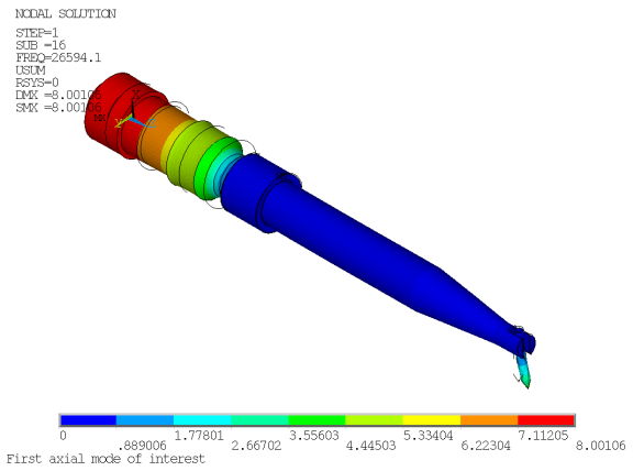
-----------------------------------------------------------------------------------------------------------------Modes having high participation factors in the z direction are candidates for evaluation as desirable longitudinal modes. Also examine the mode shapes to determine whether excessive transverse motions exist, as those modes should not be excited during transducer operation. Upon examination of the results in this case, modes 16, 30 and 39 are the modes of interest, as shown in the following three figures.
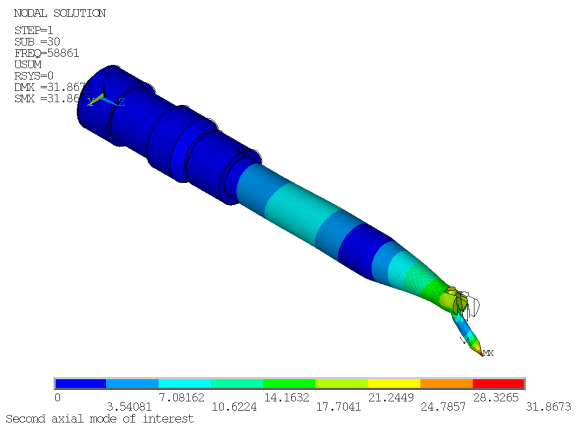
This second mode of interest is the one to be investigated in the subsequent harmonic response analyses:
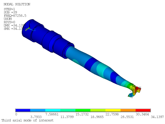
It is worth noting that if the transducer were to be used for a higher-frequency application, the third mode of interest is at 87.3 kHz:
In all modes, the tip of the bonding tool has little motion in the x and y directions as compared to the z direction, necessary for proper wire bonding to occur. Also, the frequencies of the second and third modes are roughly twice and thrice that of the first mode, as expected.
For wire bonding, the transducer can operate in the 50-60 kHz range. Although the modal analysis determined that the second longitudinal mode of interest is 58.9 kHz, it is necessary to determine the actual amplitude and impedance values, and so a harmonic response analysis is performed.
The “reaction force” for voltage degrees of freedom is charge. In
the POST26 time-history postprocessor (/POST26), the charge Q is
retrieved at the terminal. As current
 and
and
 , then
 . This operation can be performed via the CFACT
and PROD commands to calculate current based on the charge.
Impedance
. This operation can be performed via the CFACT
and PROD commands to calculate current based on the charge.
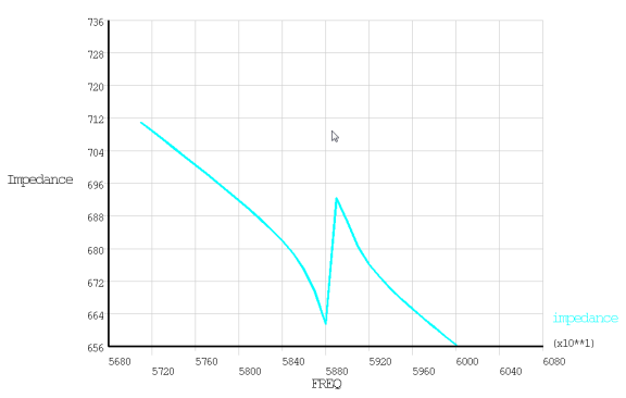
Impedance
 is calculated and plotted as follows:
The tip x, y and z displacements are output directly in POST26 and plotted as follows:
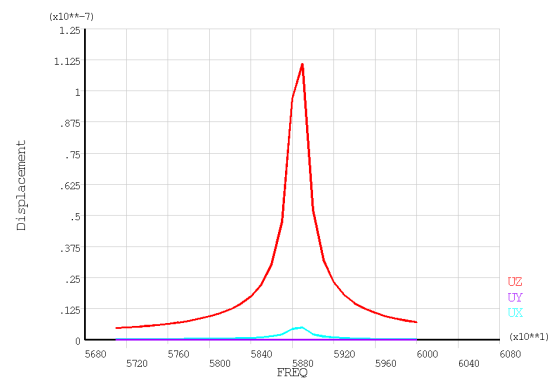
As indicated, the lateral motion (x and y) is much less than the longitudinal motion (z). The displacement for this applied voltage is a little more than 0.1 micron.