


The results are presented in terms of the four fields: structural, thermal, electrical, and diffusion.
Structural
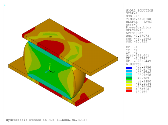
Hydrostatic stress results are in units of MPa. The gradient of hydrostatic stress produces diffusion from high to low "pressure". The stresses are due to the constraint on the top and bottom surface of the model and thermal strain incompatibility between the solder and the copper.
The figure below was produced with the command PLNSOL,NL,HPRES. A large negative hydrostatic stress occurs at the singularity produced by the sharp re-entrant corner at the edge of the solder/copper interface.
Thermal
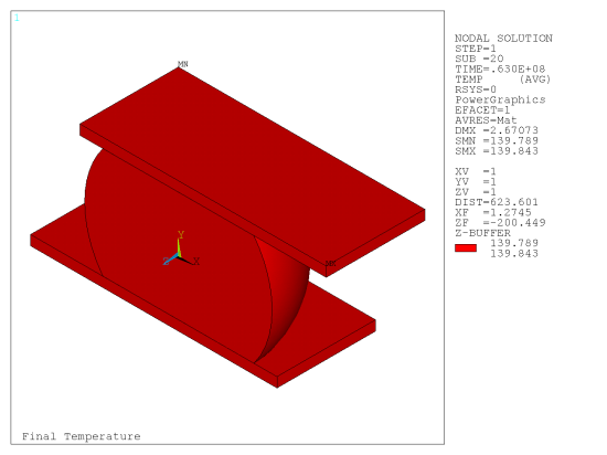
Because the model is very small and the materials have high thermal conductivity, the temperature reaches the steady-state in a few seconds and remains constant throughout the simulation. Therefore, the gradient of temperature does not contribute to atomic diffusion. The uniform temperature increase does affect diffusion by producing stress gradients due to constrained thermal expansion. The figure below was produced with the command PLNSOL,TEMP.
Electrical
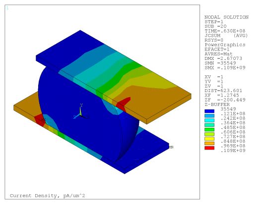
Current density is in units of pA/(μm)2 or A/m2. The figure below was produced by the command PLNSOL,JC,SUM. Note the increase in current density (current crowding) at the entrance and exit of the solder ball. This is the location where metal depletion has been observed in solder balls.
Diffusion
Regions with concentration values less than 1.0 may produce voids. Concentrations greater than 1.0 could produce hillocks or protrusions of metal from the surface. The figure below was produced with the command PLNSOL,CONC for the solder joint nodes.

Figure 47.8: Minimum Concentration vs. Time and Figure 47.9: Maximum Concentration vs. Time show the evolution of minimum and maximum concentrations with time, respectively.
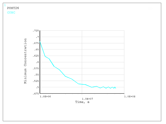
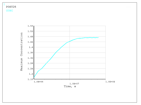
The concentration plots show that the steady state occurs after 1 year (or around time = 3x10⁷ sec).