


The shell element model gives accurate stresses in most regions; however, through-the-thickness stresses are not as accurate, especially where the reinforcement joins with the nozzle body. Solid elements are used for this analyses to improve the accuracy of through-the-thickness stresses. This problem therefore demonstrates some of the features of the solid layered thermal elements (SOLID279). The geometry for this example problem has already been meshed and stored in a cdb file.
For this example, it is assumed that the material behavior is orthotropic (both structurally and thermally). As such, it is important to define material properties along certain orthogonal directions within the elements. This underscores the need to define an element coordinate system within each element. While there is a good argument for defining material directions independent of the underlying elements, this is currently restricted by the available technology.
All elements have default element coordinate systems, but these defaults may not always be convenient. Material directions could be misaligned with respect to the element coordinate system (ESYS) and, as such, you may need to modify them. You can typically accomplish this with the following steps:
Define the element coordinate system - Due to rapidly changing curvature, each element in this model must have its own element coordinate system defined. (Consider using LOCAL and EMODIF commands for a given brick mesh.) As a result, the element z axis is aligned with the thickness direction, and the element x axis is aligned with the curvature. This makes it very convenient to define material properties along preferred directions.
Adjust the element connectivity - Because solid elements are being used, you must adjust the element connectivity so that the IJKL face is aligned with the element coordinate z axis. This ensures that the layer definition is parallel to face 1 (the IJKL face normal n) of the element and is normal to the ESYS z axis. (Consider using EORIENT to accomplish this for any arbitrary mesh with a defined element coordinate system.)

Both of these steps have already been accomplished for the model provided in this example.
Thermal stresses can be obtained using an element with TEMP and DISP degrees of freedom (DOFs) that are fully coupled (strong coupling). Alternately, stresses can be obtained using a thermal run and then a structural run (loose coupling). The advantages and disadvantages of these methodologies are not fully detailed here. Instead, this example uses the loose coupling method to demonstrate the flexibility that it offers.
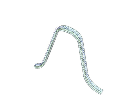
In this example a static thermal analysis is run using element SOLID279, and then temperatures are transferred to a static structural analysis using the LDREAD command. For the structural run, SOLID279 is converted into SOLID186. For the thermal run, it is assumed that the material can be homogeneous or layered. A similar assumption is made for the structural run, therefore allowing you to use the temperatures from either a homogeneous or layered run for a structural run, as illustrated in the figure below:

A material could be treated as homogeneous for a thermal run and layered for a structural run. This allows you the flexibility to mix and match the runs at your own discretion. A strongly coupled solution would not provide this level of flexibility and freedom.