


Curve-fitting is performed for data from a strain-controlled stable hysteresis loop, as well as for data from a stress-controlled loop, and then for the combined set of data. The experimental data is taken from Bari and Hassan [4]. The initial parameters are estimated as described in Determining Material Parameters.
To verify that the parameters from the curve-fitting tool give a good match to experimental data over the entire loading history, uniaxial single-element tension-compression simulations are performed.
The following related topics are available:
The curve-fitting and simulation portions of the uniaxial strain-controlled experiment are described here.
The initial parameters are determined using the experimental strain-controlled data. .
Because the initial yield stress for the material is well known, the value is fixed.
The value for γ3 does not significantly affect the model predictions for the stable hysteresis loop, and it is best fit to cyclic stress ratcheting data. In this problem, the value is fixed because allowing it to vary in the fitting procedure produced a poor set of material coefficients.
The following table shows the initial parameters and those determined via the curve-fitting tool:
Table 31.1: Initial and Fitted Parameters for the Strain-Controlled Experiment
| Parameter | Initial Parameters | Fitted Parameters |
|---|---|---|
| C1 (ksi) | 60000 | 5174000 |
| γ1 | 20000 | 4607500 |
| C2 (ksi) | 13850 | 17155 |
| γ2 | 996.1 | 1040 |
| C3 (ksi) | 450 | 895.18 |
| γ3 | 9 | 9 |
| σ0 (ksi) | 18.8 | 18.8 |
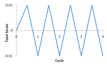
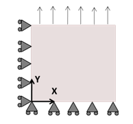
To simulate the loading history over the entire uniaxial strain-controlled experiment, a single SOLID185 element is used with quarter symmetry boundary conditions and uniaxial displacement in the Y direction. Elastic properties are a Young’s modulus of 26300 ksi and a Poisson’s ratio of 0.302. The nodes are given a displacement value to simulate a strain cycle with an amplitude of 0.01.
The following figure shows the loading history for the entire experiment:
This figure shows a schematic of the model:
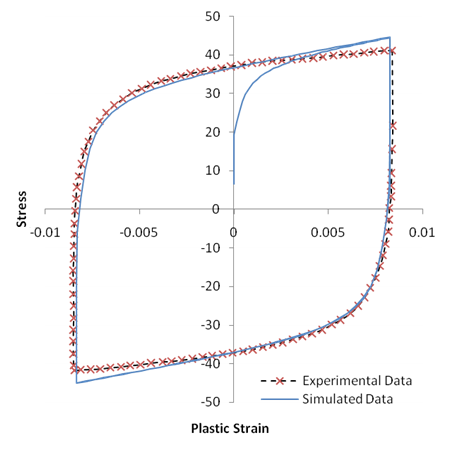
The following table compares the simulated results at the maximum negative plastic strain to the experimental data:
Table 31.2: Comparison of Strain-Controlled Experimental Data with Simulated Data
| Simulated | Experimental | Ratio | |
|---|---|---|---|
|
Maximum Stress (ksi) | 43.6 | 41.1 | 1.06 |
|
Plastic Strain at Maximum Stress | 0.00829 | 0.00837 | 0.990 |
Following is a plot of the stress-strain history:
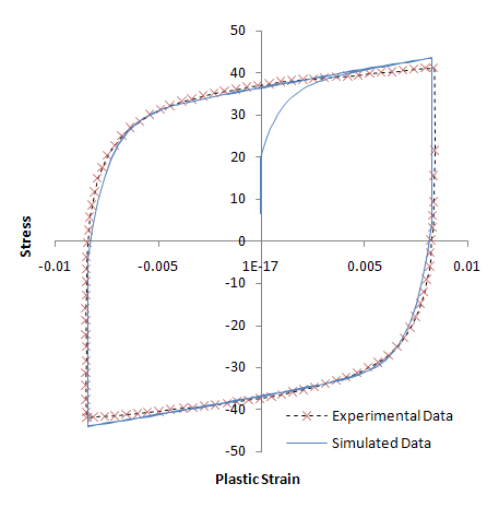
The model predictions indicate that little evolution occurs in the stress-strain plot after the initial cycle and the hysteresis loop has stabilized. If the hysteresis continues to evolve over several loading cycles, the model prediction from the curve-fitting tool will not correspond to the stabilized hysteresis predicted by the model.
To alleviate the inconsistency, try inputting multiple copies of the same experimental data. The curve-fitting algorithm can then minimize the error from the model prediction over multiple cycles.
The curve-fitting and simulation portions of the uniaxial stress-controlled experiment are described here.
The initial parameters are determined using the stress-controlled experimental data from Bari and Hasan [4]. The following table shows the initial parameters and those determined via the curve-fitting tool:
Table 31.3: Initial and Fitted Parameters for the Stress-Controlled Experiment
| Parameter | Initial Parameters | Fitted Parameters |
|---|---|---|
| C1 (ksi) | 100000 | 29214 |
| γ1 | 10000 | 4608.9 |
| C2 (ksi) | 10000 | 11315 |
| γ2 | 1000 | 1261.8 |
| C3 (ksi) | 1000 | 1517.8 |
| γ3 | 10 | 10 |
| σ0 (ksi) | 18.8 | 18.8 |
While the heuristic procedure for determining the initial parameters was developed for stabilized hysteresis strain-controlled data, using the procedure on a single load cycle of stress-controlled data often gives an adequate set of initial parameters. It may be necessary to adjust the initial parameters, however, if a good fit is not evident after comparing the results from the fitted model to the experimental data.
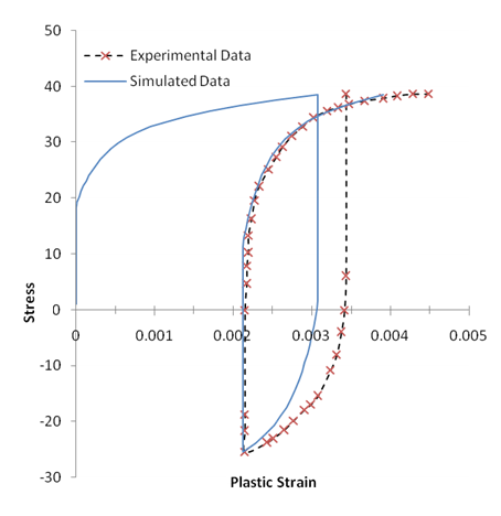
The same finite element model is used as that for the simulation of the strain-controlled experiment. The loading is changed to a uniaxial stress cycle between 38.68 ksi and -25.45 ksi. The results from the single element simulation are compared with the experimental data in the following figure:
The curve-fitting tool can use more than one data set in the fitting procedure. The stabilized hysteresis data has been used to estimate the initial parameters. The curve-fitting tool then uses both the stabilized hysteresis and stress-controlled experimental data to generate the fitted parameters. The following table shows the initial and fitted parameters:
Table 31.4: Initial and Fitted Parameters for Fit to Both Data Sets
| Parameter | Initial Parameters | Fitted Parameters |
|---|---|---|
| C1 (ksi) | 60000 | 26291 |
| γ1 | 20000 | 2409.8 |
| C2 (ksi) | 13850 | 3781.0 |
| γ2 | 996.1 | 537.58 |
| C3 (ksi) | 450 | 976.46 |
| γ3 | 9 | 9 |
| σ0 (ksi) | 18.8 | 18.8 |
The comparison of the experimental data sets and the model predictions data for the fit to multiple data sets are shown in the following two figures:
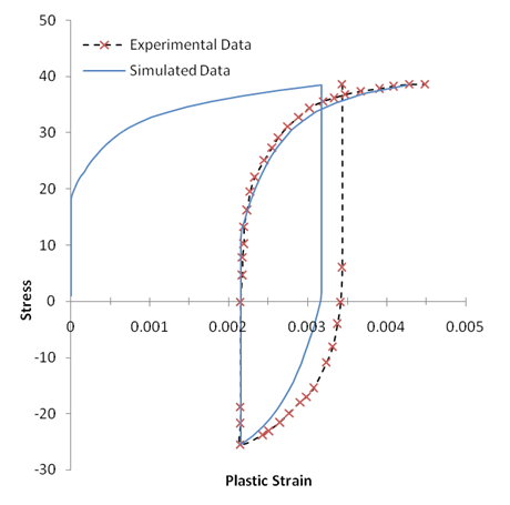
The stabilized hysteresis comparison shows a slightly better fit in the unloading knee and a change in the data fit for the loading knee. The predictions at the maximum and minimum plastic strain points are not significantly affected, however. The stress-controlled data comparison also shows a shift in the reloading knee region, but the plastic strain prediction in the initial unloading point still shows significant error.
Using the three backstress components to fit the three parts of the stress-strain behavior (as described in Determining Material Parameters), it is difficult to fit the value of γ3 using either the stabilized hysteresis or the stress-controlled data. The value of γ3, however, can be used to match the rate at which plastic strain accumulates over a number of loading cycles.
The following figure shows data from Bari and Hassan [4] that illustrates the accumulation of plastic strain over 45 cycles of loading:
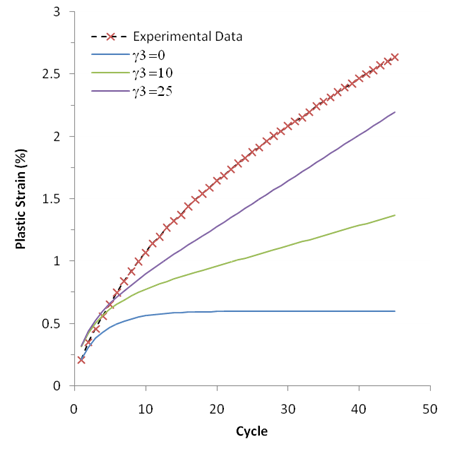
The load cycle is the same as that used for the stress-controlled data. Also shown are predictions from the model using the parameters from the fit to multiple data sets, except that three different values for γ3 are used. The plot shows that the rate of plastic strain accumulation after about 10 cycles of loading is nearly linear with the value of γ3 controlling this rate of ratcheting.
For a value γ3 = 25, the rate of ratcheting approximately matches the experimental data; however, the total amount of plastic strain from the model does not match the experimental data. One reason is that the plastic strain in the early part of the load history is affected by the isotropic hardening behavior, which quickly saturates after a few loading cycles.
Selecting a value for γ3 to match the ratcheting rate is a manually iterative process, as a fixed value is set and a new fit to the other Chaboche parameters is obtained via the curve-fitting tool.