Commonly used plasticity models for ratcheting are based on the von Mises yield criterion and a kinematic hardening rule. The von Mises yield criterion for kinematic hardening is:
 | (31–1) |
where  is the isotropic hardening yield stress, and
  is the center of the yield surface which is a function of the
stress tensor
is the center of the yield surface which is a function of the
stress tensor  and backstress tensor
  :
:

The backstress tensor results in a shifting of the yield surface in stress space. A bias in this shift over repeated loading causes the progressive accumulation of plastic strain (ratcheting).
Experimental data and the curve-fitting tool are used to determine a set of material parameters for the Chaboche kinematic hardening model. A third-order Chaboche kinematic hardening model is used, as it provides sufficient variation to calibrate the nonlinear behavior of the material and can account for ratcheting behavior. More parameters can be used but, for the data used in this problem, a third order is sufficient.
The following related topics are available:
Chaboche [1][2] proposed the decomposed kinematic hardening model, expressed as:
 | (31–2) |
 | (31–3) |
where:

Each of the backstress terms of the Chaboche model have the form of an
Armstrong-Frederick rule, where the parameters  represent a plastic modulus and
  serve as the parameters for history dependence. For accurate
ratcheting predictions, specify at least three components [3].
serve as the parameters for history dependence. For accurate
ratcheting predictions, specify at least three components [3].
For a stable hysteresis of strain-controlled cyclic loading, the solution for the backstress in the uniaxial direction is:
 | (31–4) |
 | (31–5) |
where:

The uniaxial yield stress is the sum of the initial yield stress and the backstress component in the uniaxial direction, expressed as:
 | (31–6) |
Using Equation 31–4 and Equation 31–5 for
plastic strains at or near the strain limit
 , Equation 31–6 for a third-order Chaboche
model becomes:
, Equation 31–6 for a third-order Chaboche
model becomes:
 | (31–7) |
The model requires six material parameters: C1, γ1, C2, γ2, C3, and γ3 as well as the initial yield stress, σ0.
The parameters must be determined so that the model closely matches the material behavior. One method for doing so is to obtain data from stabilized strain-controlled and stress-controlled ratcheting experiments and use that data with the curve-fitting tool to determine material parameters that minimize the error between the data and the model predictions.
The nonlinear curve-fitting method used by the curve-fitting tool is an iterative process and requires initial values for each of the material parameters. The success and quality of the fit depends on how far the initial values are from the values that give a good fit. A procedure is developed using stabilized hysteresis stress-strain data to determine a good estimate for the initial parameters.
Stabilized hysteresis stress-strain data is obtained by cycling a specimen under strain-controlled loading with symmetric tension-compression amplitude. A cyclically stabilized hysteresis response is achieved when a cycle of stress-strain response remains unchanged through subsequent cycles.
The following figure shows a typical stable strain-controlled hysteresis curve:
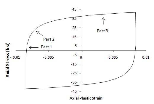
Three distinct regions are noted. Part 1 is the initial onset of yielding, Part 2 is the knee of the hysteresis curve, and Part 3 is the constant modulus segment.
For fitting purposes, the individual components of backstress for the model (α1, α2, and α3) are chosen to represent the three regions of the strain-controlled stable hysteresis loop. In each region, the corresponding Ci is chosen to approximately match the plastic modulus. The γi parameters are chosen to accommodate the history dependence defined by Equation 31–4 and the relationship defined by Equation 31–7.
Using the described heuristic method, the initial material parameters can be estimated as follows:
σ0 is the initial yield stress of the material.
C1 is the slope in Part 1 of the stress-strain curve at the transition from elastic to plastic deformation. This value is approximately the plastic modulus at yielding.
Using Equation 31–4, γ1 should be large enough that the exponential term quickly diminishes so that α1 is approximately constant outside of Part 1.
C2 is chosen as a slope from Part 2.
γ2 is calculated from the chosen C2 and the ratio C2 / γ2 that satisfies Equation 31–7.
C3 is the slope of the stress-strain curve in Part 3.
γ3 is not included in Equation 31–4 through Equation 31–7 and is assigned a small positive value.
The procedure was developed from a trial-and-error method used to fit the material parameters [4] and usually gives a set of initial parameters that allows the curve-fitting tool to obtain a good fit.
The initial yield stress of the material is generally known, and in this problem it is fixed and does not affect the error minimization performed by the curve-fitting tool.
γ3 is chosen as a small positive value because it does not enter into the closed-form equations, and experience indicates that this is generally a good choice. While the fitting procedure iterates to a value of γ3 that best fits the data, this value is often difficult to estimate based on stabilized hysteresis strain-controlled data. The value of this parameter affects the amount of ratcheting in each cycle of a stress-controlled experiment and is best determined using that data.
Although the procedure for estimating the initial material parameters was developed for stabilized hysteresis strain-controlled data, it can be applied to a single cycle of stress-controlled data; however, the quality of the resulting fit should be checked carefully.
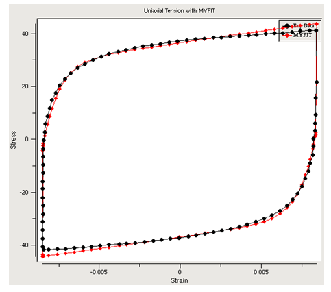
The curve-fitting tool provides a comparison of the data used for fitting and the model's prediction. It is good practice, however, to compare the experimental data with a simulation of the entire experimental load history to validate the fitted parameters, as shown in this figure: