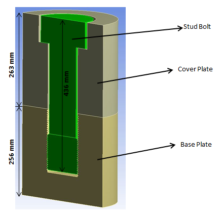
The two primary characteristics in a bolted joint are pretension and mating part contact. To simulate the bolt configuration, a stud M120 bolt is modeled with a cover and a base plate. The bolt is subjected to a pretension load of 256446 N to simulate the actual bolt phenomenon. Three frictional contact pairs (FCP) are defined: one in the thread region, another between the bolt head and the cover plate, and the third between the cover plate and the base plate.
A pressure load of 50 MPa (which is less than the equivalent pretension load) is applied to the upper surface of the cover plate after applying pretension to the bolt. The resulting bolt shank stress (stress in the region between the bolt head and the bolt thread) due to the pretension load and the inclusion of frictional contact behavior are the major concerns during the bolt simulation.
The objective of this problem is to show that the bolt section method simplifies the modeling of this bolt joint and produces approximate thread behavior and shank stress that are comparable to the true threaded bolt model.
This problem is simulated by three methods:
True thread simulation
This method is the most accurate bolt simulation. The detailed modeling of threads provides accurate thread behavior in the model. Very refined mesh discretization is required in the thread region, which makes this method computationally expensive.
Bolt section method (simplified bolt thread modeling technique)
In this method, the bolt thread is simulated by assigning a bolt section to the contact elements overlaid on the smooth cylindrical bolt surface. (No detailed thread geometry is required.) Calculations are performed internally based on the thread parameters given by the SECDATA command to approximate the behavior of the bolt. This method is computationally inexpensive.
MPC method (bonded behavior in thread region)
In this method, MPC bonded behavior is defined in the thread region. (No detailed thread geometry is required.) This method is very fast computationally, but thread behavior can be lost.
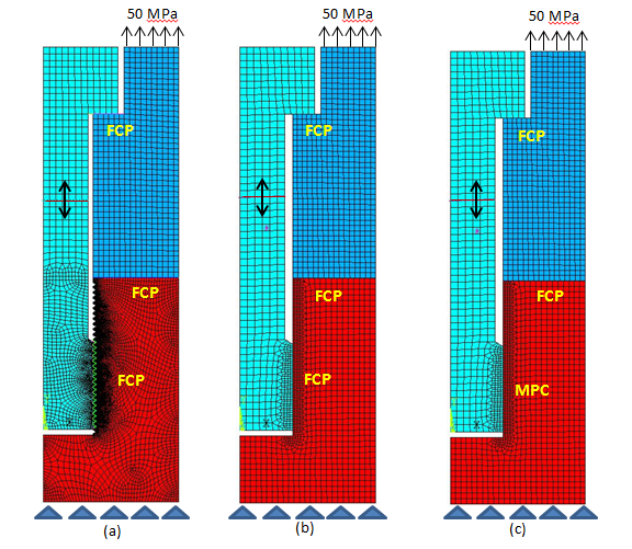
Both 2D axisymmetric and 3D models are used to compare these three methods. The 2D model setup for all three methods is shown in the figure below.
Figure 37.2: 2D Axisymmetric Problem Setup for (a) True Thread, (b) Bolt Section, (c) MPC Bonded Method