


The basic equation solved in a typical undamped modal analysis is the classical eigenvalue problem:

where:
| [K] = stiffness matrix |
| {Φi} = mode shape vector (eigenvector) of mode i |
Ωi = natural circular frequency of mode i
(
 is the eigenvalue) is the eigenvalue) |
| [M] = mass matrix |
Many numerical methods are available to solve the equation. Mechanical APDL offers these methods:
The damped and QR damped methods solve different equations. For more information, see Damped Method and QR Damped Method in the Mechanical APDL Theory Reference.
Table 3.5: Symmetric System Eigensolver Options
| Eigensolver | Application | Memory Required | Disk Required |
|---|---|---|---|
| Block Lanczos | To find many modes (about 40+) of large models. Recommended when the model consists of poorly shaped solid and shell elements. This solver performs well when the model consists of shells or a combination of shells and solids. | Medium | High |
| PCG Lanczos | To find few modes (up to about 100) of very large models (1,000,000+ degrees of freedom). This solver performs well when the lowest modes are sought for models that are dominated by well-shaped 3D solid elements (that is, models that would typically be good candidates for the PCG iterative solver for a similar static or full transient analysis). | Medium | Low |
| Supernode | To find many modes (up to 10,000) efficiently. Use this method for 2D plane or shell/beam structures (100 modes or more) and for 3D solid structures (250 modes or more). | Medium | Low |
| Subspace | To find many modes (about 40+) of large models. This solver is more robust when the mass matrix is partially zero, or when there are u-P formulation elements in the model. It is recommended when using distributed-memory parallel processing. | Medium | High |
The Block Lanczos eigenvalue solver uses the Lanczos algorithm where the Lanczos recursion is performed with a block of vectors. The Block Lanczos method uses the sparse matrix solver, overriding any solver specified via EQSLV.
The Block Lanczos method is especially powerful when searching for
eigenfrequencies in a given part of the eigenvalue spectrum of a given system. The
convergence rate of the eigenfrequencies will be about the same when extracting
modes in the midrange and higher end of the spectrum as when extracting the lowest
modes. Therefore, when you use a shift frequency (FREQB
on MODOPT) to extract n modes
beyond the starting value of FREQB, the algorithm
extracts the n modes beyond
FREQB at about the same speed as it extracts the
lowest n modes.
While the Block Lanczos eigensolver is typically very robust for a wide range of applications, some element types may cause the eigensolver difficulty in achieving a final solution. These include MPC184 elements that use the Lagrange multiplier method and FLUID30, FLUID220, and FLUID221 elements that use the symmetric element matrix formulation for modal analyses (KEYOPT(2) = 2).
The PCG Lanczos method internally uses the Lanczos algorithm, combined with the PCG iterative solver. This method is significantly faster than the Block Lanczos method in the following cases:
Large models that are dominated by 3D solid elements and do not have ill-conditioned matrices due, for example, to poorly shaped elements
Only a few of the lowest modes are requested
Having ill-conditioned matrices or asking for many (say, more than 100) modes can lead to a long solution time.
The PCG Lanczos method finds only the lowest eigenvalues. If a range of eigenfrequencies is requested (MODOPT), the PCG Lanczos method finds all eigenfrequencies below the lower value of the eigenfrequency range as well as the number of requested eigenfrequencies in the given eigenfrequency range. The PCG Lanczos method is therefore not recommended for problems when the lower value of the input eigenfrequency range is far from zero.
When to Use PCG Lanczos over Block Lanczos
The Block Lanczos eigensolver is the recommended eigensolver for most applications; however, the PCG Lanczos eigensolver can be more efficient than the Block Lanczos eigensolver for certain cases. Follow these guidelines when deciding whether to use the Block Lanczos or PCG Lanczos eigensolver.
Typically, the following conditions must be met for the PCG Lanczos eigensolver to be most efficient:
The model would be a good candidate for using the PCG solver in a similar static or full transient analysis.
The number of requested modes is less than a hundred.
The beginning frequency input via MODOPT is zero (or near zero).
The PCG Lanczos eigensolver (like all iterative solvers) is most efficient when the solution converges quickly. If the model does not converge quickly in a similar static or full transient analysis, it is expected that the PCG Lanczos eigensolver will also not converge quickly and will therefore be less efficient. The PCG Lanczos eigensolver is most efficient when finding the lowest natural frequencies of the system. (For detailed information on measuring PCG Lanczos solver efficiency, see PCG Lanczos Solver Performance Output in the Performance Guide.) As the number of requested modes begins to approach one hundred, or when requesting only higher modes, the Block Lanczos eigensolver becomes a better choice.
Other factors such as the size of the problem and the hardware being used can
affect the eigensolver selection strategy. For example, when solving problems where
the Block Lanczos eigensolver runs in an out-of-core mode on a system with very slow
hard drive speed (that is, bad I/O performance) the PCG Lanczos eigensolver may be
the better choice as it does significantly less I/O, assuming a
Lev_Diff value of 1 through 4 is used
(PCGOPT). Another example would be solving a model with 15
million degrees of freedom. In this case, the Block Lanczos eigensolver would need
approximately 300 GB of hard drive space. If computer resources are limited, the PCG
Lanczos eigensolver may be the only viable choice for solving this problem since the
PCG Lanczos eigensolver does much less I/O than the Block Lanczos eigensolver. The
PCG Lanczos eigensolver has been successfully used on problems exceeding 100 million
degrees of freedom.
The Supernode (SNODE) solver is used to solve large, symmetric eigenvalue problems for many modes (up to 10,000 and beyond) in one solution. Typically, the reason for seeking many modes is to perform a subsequent mode-superposition or PSD analysis to solve for the response in a higher frequency range.
A supernode is a group of nodes from a group of elements. The supernodes for the
model are generated automatically by the program. This method first calculates
eigenmodes for each supernode in the range of 0.0 to FREQE*RangeFact (where RangeFact is
specified via SNOPTION and defaults to 2.0), and then uses the
supernode eigenmodes to calculate the global eigenmodes of the model in the range of
FREQB to FREQE (where FREQB and
FREQE are specified via
MODOPT).
Typically, this method offers faster solution times than Block Lanczos or PCG Lanczos if the number of modes requested is more than 200. The accuracy of the Supernode solution can be controlled by SNOPTION. For more information, see Supernode Method in the Theory Reference.
The lumped mass matrix option (LUMPM,ON) is not allowed when using the Supernode mode-extraction method. The eigensolver will automatically be switched to Block Lanczos in this case.
When to Use Supernode
Typically, the following conditions must be met for the Supernode eigensolver to be most efficient:
The model is a good candidate for using the sparse solver in a similar static or full transient analysis (that is, the model is dominated with beams/shells or has a thin structure).
The number of requested modes is greater than 200.
The beginning frequency input via MODOPT is zero (or near zero).
For models that are dominated by solid elements or have a bulkier geometry, the Supernode eigensolver can still be more efficient than other eigensolvers; however, it may require higher numbers of modes to become the best choice in terms of performance. Other factors, such as the hardware being used, can also affect the decision of which eigensolver to use. For example, on machines with slow I/O performance the Supernode eigensolver may be the faster eigensolver (compared to Block Lanczos).
The Subspace method is an iterative algorithm that is appropriate for problems
having symmetric stiffness and mass matrices ( and
and  ). It internally uses the sparse solver for the shift-invert logic.
The Subspace solver performs well when the goal is to obtain a moderate to medium
number of eigenvalues on large models run in distributed parallel mode.
). It internally uses the sparse solver for the shift-invert logic.
The Subspace solver performs well when the goal is to obtain a moderate to medium
number of eigenvalues on large models run in distributed parallel mode.
Sturm sequence checking (off by default) is available for this method and is controlled via SUBOPT. The command can also control memory usage of the algorithm.
The unsymmetric method, which also uses the
full  and
and  matrices, is meant for problems where the stiffness and mass
matrices are unsymmetric (for example, acoustic fluid-structure interaction
problems). Sturm sequence checking is not available for this method. Therefore,
missed modes are a possibility at the higher end of the frequencies
extracted.
matrices, is meant for problems where the stiffness and mass
matrices are unsymmetric (for example, acoustic fluid-structure interaction
problems). Sturm sequence checking is not available for this method. Therefore,
missed modes are a possibility at the higher end of the frequencies
extracted.
Solutions from the unsymmetric method can be real or complex. By default, the
solution type is determined automatically (Cpxmod = AUTO
on MODOPT).
For details about the complex frequency definition, see Complex Eigensolutions in the Theory Reference. For details about complex solution postprocessing, see POST1 and POST26 – Complex Results Postprocessing in the Theory Reference.
The damped method
(MODOPT,DAMP) is meant for problems where damping cannot be
ignored, such as rotor dynamics applications. It uses the full matrices
( ,
,  , and the damping matrix
  ).
).
Sturm sequence checking is not available for this method. Therefore, modes may be missing in the higher end of the range of extracted frequencies.
In a damped system, the eigensolutions are complex and the response at different nodes can be out of phase. At any given node, the amplitude will be the vector sum of the real and imaginary components of the eigenvector.
The complex frequencies are generally pairs of complex conjugates except in cases where system matrices are unsymmetric and structural damping is present.
For an example showing the use of the MODOPT and DAMPOPT commands to extract eigenvalues within a frequency range of interest, see Example: Shift Option Usage on DAMPOPT. For details about the complex frequency definition, see Complex Eigensolutions in the Theory Reference. For details about complex solution postprocessing, see POST1 and POST26 – Complex Results Postprocessing in the Theory Reference.
3.8.6.1. Example: Shift Option Usage on DAMPOPT
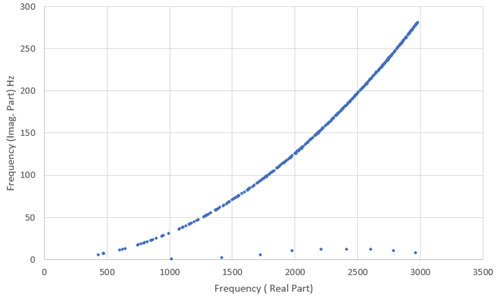
Consider an example having many complex eigenfrequencies with the real part in the range of 0 to 3000 Hz. Using the sequence of commands below, eigenvalues are reported as shown in Figure 3.2: Eigenfrequency Spectrum with the SHIFT Option, First 1000.
/solu
antype,modal
modopt,damp,1000,10,3000  ! Request the first 1000 eigenvalues
                          !   in the range 10 to 3000 Hz
dampopt,shift,on          ! Activate the shift option
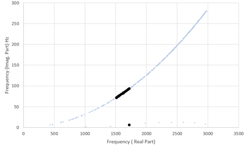
Using the following command input, you can ask for only the eigenfrequencies within a frequency range starting at 1500 Hz. The result is shown in Figure 3.3: Subset of Eigenfrequencies with the SHIFT Option. The black points on the graph show the resulting subset of eigenfrequencies compared to the above case of 1000 requested eigenvalues.
/solu
antype,modal
modopt,damp,20,1500   ! Only request the first 20
                      !   eigenvalues > 1500 Hz
dampopt,shift,on      ! Activate the shift option
                      ! The DAMP algorithm uses a shift
                      !   of 1500 Hz to initiate the search
Note that when the SHIFT option is active and FREQB
is specified, the damped eigensolver only produces eigenfrequencies with a real
part greater than FREQB. If
FREQB is not specified, the damped eigensolver
finds eigenvalues closest to the 0 Hz point.
The QR damped method (MODOPT,QRDAMP) combines the advantages of a symmetric eigensolution method with the complex Hessenberg method. The key concept is to approximately represent the complex damped eigenvalues by modal transformation using a larger number of eigenvectors of the undamped system. After the undamped mode shapes are evaluated by using the real eigensolution, the equations of motion are transformed to these modal coordinates.
Using the QR algorithm, a smaller eigenvalue problem is then solved in the modal subspace. This approach gives good results for lightly damped systems and can also apply to any arbitrary damping type: proportional or non-proportional symmetric damping, nonsymmetrical gyroscopic damping matrix, or structural damping. It is recommended to use the Damp eigensolver (MODOPT,DAMP) when the complex eigenvalues are not conjugate pairs as only half of them are output by the QRDAMP eigensolver. Such cases include, but are not limited to:
structural damping and unsymmetric system matrices
a mix of viscous and structural dampings.
The QRDAMP eigensolver applies to models having an unsymmetrical global stiffness matrix where only a few elements contribute unsymmetric element stiffness matrices. For example, in a brake-friction problem, the local part of a model with friction contacts generates a unsymmetric stiffness matrix in contact elements. When an unsymmetric stiffness matrix is encountered, the eigenfrequencies and mode shapes obtained by the QRDAMP eigensolver should be verified by rerunning the analysis with the unsymmetric eigensolver. If an unsymmetric stiffness matrix is encountered, the QRDAMP eigensolver issues a message after completing the symmetric eigensolution.
The QRDAMP eigensolver works best when there is a larger modal subspace to converge and is therefore the best option for larger models. Because the accuracy of this method is dependent on the number of modes used in the calculations, a sufficient number of fundamental modes should be present (especially for highly damped systems) to provide good results. The QR damped method is not recommended for critically damped or overdamped systems. This method outputs both the real and imaginary eigenvalues (frequencies). By default, only the real eigenvectors (mode shapes) are output, although complex mode shapes can be calculated if needed (MODOPT).
Additional QRDAMP eigensolver options can be set via QRDOPT.
In general, Ansys, Inc. recommends using the Damp eigensolver for small models. It produces more accurate eigensolutions than the QR Damped eigensolver for damped systems.
For details about the complex frequency definition, see Complex Eigensolutions in the Theory Reference. For details about complex solution postprocessing, see POST1 and POST26 – Complex Results Postprocessing in the Theory Reference.