


After you have run a modal analysis with several rotational velocity load steps, you can perform a Campbell diagram analysis. The analysis allows you to:
Visualize the evolution of the frequencies with the rotational velocity
Determine the critical speeds.
Determine the stability threshold
The plot showing the variation of frequency with respect to rotational velocity may not be readily apparent. For more information, see Generating a Successful Campbell Diagram below.
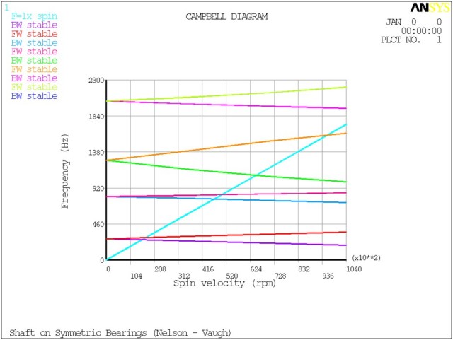
In the general postprocessor (POST1), issue the PLCAMP command to display a Campbell diagram as shown below.
If there are rotating components, you will specify the name of the reference
component via the Cname argument in the
PLCAMP command.
A maximum of 10 frequency curves are plotted within the frequency range specified.
Use the following commands to modify the appearance of the graphics:
- Scale
To change the scale of the graphic, you can use the /XRANGE and /YRANGE commands.
- High Frequencies
Use the FREQB argument in the PLCAMP command to select the lowest frequency of interest.
- Rotational Velocity Units
Use the UNIT argument in the PLCAMP command to change the X axis units. This value is expressed as either rd/sec (default), or rpm.
Use the SLOPE argument in PLCAMP command to display the line representing an excitation. For example, an excitation coming from unbalance corresponds to SLOPE = 1.0 because it is synchronous with the rotational velocity.
Forward (FW), and backward (BW) whirls, and unstable frequencies are identified in the Campbell diagram analysis. These characteristics appear in the Campbell diagram graphic legend generated by the PLCAMP command. Forward and backward whirls are printed out in the table generated by the PRCAMP command, as shown below.
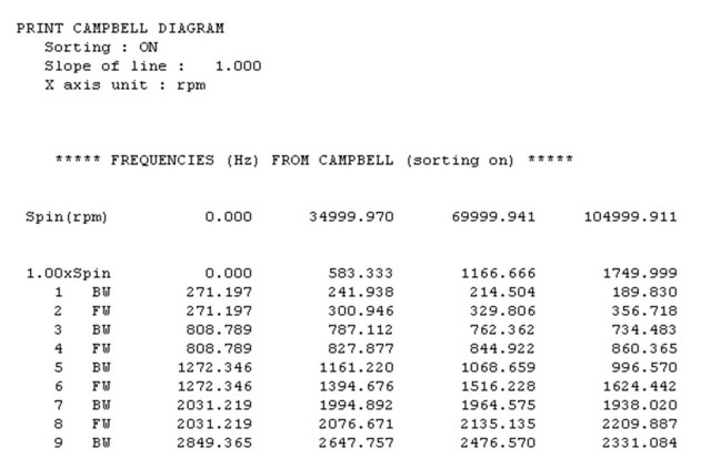
If an unstable frequency is detected, it is identified in the table by a letter u between the mode number and the whirl characteristics (BW/FW). In this example, all frequencies are stable.
The whirl direction is calculated at maximum rotational
velocity by default. KeyWhirl on the
PRCAMP command can be used to print out the whirl direction
of each mode at each rotational velocity. The whirl direction of a mode is
calculated as the average of the whirl directions of the nodes belonging to a
rotating part. The nodal whirl directions can be printed out using
WhrlNodkey = ON on the PRORB
command.
Note: For a rotating structure meshed in shell elements lying in a plane perpendicular to the rotational velocity axis—for example, a thin disk—the whirl effects are not plotted or printed by the PRCAMP or PLCAMP commands. However, they can be visualized using the ANHARM command.
By default, the PRCAMP command prints a maximum of 10
frequencies (to be consistent with the plot obtained via the
PLCAMP command). If you want to see all frequencies, set KeyALLFreq = 1.
You can determine how a particular frequency becomes unstable by issuing the PLCAMP or PRCAMP and then specifying a stability value (STABVAL) of 1. You can also view the logarithmic decrements by specifying a STABVAL = 2 or 3.
To retrieve and store frequencies and whirls as
parameters: Use the *GET command with
Entity = CAMP and Item1 =
FREQ or WHRL. A maximum of 200 values are retrieved within the frequency range
specified.
The PRCAMP command prints out the critical speeds for a rotating synchronous (unbalanced) or asynchronous force when SLOPE is input:
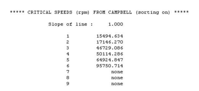
The critical speeds correspond to the intersection points between frequency curves and the added line F = sω (where s represents SLOPE > 0 as specified via PRCAMP).
Because the critical speeds are determined graphically, their accuracy depends upon the quality of the Campbell diagram. For example, if the frequencies show significant variations over the rotational velocity range, you must ensure that enough modal analyses have been performed to accurately represent those variations. For more information about how to generate a successful Campbell diagram, seeGenerating a Successful Campbell Diagram below.
To retrieve and store critical speeds as parameters:
Use the *GET command with
Entity = CAMP and Item1 =
VCRI. A maximum of 200 values are retrieved within the frequency range
specified.
The PRCAMP command prints out the stability threshold of each
mode when a zero line (SLOPE) is input and stability
values (or logarithmic decrements) are post-processed
(STABVAL = 1, 2, or 3).
Stability thresholds correspond to change of signs. Because they are determined graphically, their accuracy depends upon the quality of the Campbell diagram. For example, if the stability values (or logarithmic decrements) show significant variations over the rotational velocity range, you must ensure that modal analyses have been performed with enough load steps to accurately represent those variations.
To retrieve and store stability thresholds as parameters, use the
*GET command with Entity = CAMP
and Item1 = VSTA.
To help you obtain a good Campbell diagram plot or printout, the sorting option is active by default (PLCAMP,ON or PRCAMP,ON). The program compares complex mode shapes obtained at 2 consecutive load steps using the Modal Assurance Criterion (MAC). The equations used are described in POST1 - Modal Assurance Criterion (MAC) in the Mechanical APDL Theory Reference. Similar modes shapes are then paired. If one pair of matched modes has a MAC value smaller than 0.7, the following warning message is output:
*** WARNING ***
Sorting process may not be successful due to the shape of some modes.
If results are not satisfactory, try to change the load steps and/or
the number of modes.
In this case, or if the plot is otherwise unsatisfactory, try the following:
Start the Campbell analysis with a nonzero rotational velocity.
Modes at zero rotational velocity are real modes and may be difficult to pair with complex modes obtained at nonzero rotational velocity.
Increase the number of load steps.
It helps if the mode shapes change significantly as the spin velocity increases.
Change the frequency window.
To do so, use the shift option (PLCAMP,,,
FREQBor PRCAMP,,,FREQB). It helps if some modes fall outside the default frequency window.
Running multiple damped modal analyses for a 3D model may result in a large results file. To reduce its size, you can:
Decrease the number of extracted modes (MODOPT,,NMODE).
Generate the results file for a reduced set of selected nodes (for example, nodes on the axis of rotation). Issue OUTRES,ALL,NONE and then OUTRES,
Item,Freq,CnamewhereItem= NSOL,Freq= ALL andCnameis the name of a node-based component.For the sorting process and whirl calculation to be successful, the set of selected nodes must represent the dynamics of the structure. In general, nodes on the spin axis contribute to the bending mode shapes that are needed in the Campbell analysis.