The following examples are available:
This section describes a sample harmonic edge-based analysis, performed using Mechanical APDL.
This example examines the solution in the slot of an electric machine. For a specified AC (harmonic) current, the analysis calculates the magnetic field, energy, Joule heat losses and forces.
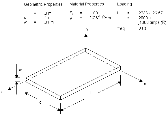
Figure 6.4: Current-Carrying Conductor in a Slot Within an Iron Region (in 3D Magnetostatics and Fundamentals of Edge-Based Analysis) and Figure 7.1: Volume Model of the Conductor illustrate, respectively, the problem domain and a volume model of the conductor within the slot in the domain.
The geometry is a block modeling a slot of an electrical machine. The z-axis coincides with the axis of the machine; l = .3 m is the length. The slot, with a depth of d = 0.1 m, is oriented in the x-axis. The width of the slot in the y direction is denoted by w = 0.01 m. A conductor with relative permeability, µr = 1, and resistivity, ρ = 1.0e-8, carries a current of 2236 A at a phase angle of 26.57° (corresponds in complex terms to 2000 + j1000 A). The analysis frequency is 3 Hz, which corresponds to a 5% slip frequency for a machine operating at 60 Hz.
The side and bottom of the slot are ideal iron. This is a flux-normal boundary condition (natural (Neumann) boundary condition); it is satisfied automatically without any prescription of an explicit boundary condition.
At the opening of the slot at x = d and at axial faces z = 0 and z = 1, the flux lines are parallel. This is an essential flux-parallel (Dirichlet) boundary condition; that is, its satisfaction is not automatic. You can prescribe it by setting (constraining) the flux-edge DOFs to a constant value, usually zero.
The example uses MKS dimensions (the default).
Parameters for the example are as follows:
| l = 0.3 | Length |
| d = 0.1 | Depth |
| w = 0.01 | Width |
| i = 2000 + j1000 | Current |
| mur = 1 | Relative magnetic permeability |
| ρ = 1.0e-8 | Electric resistivity (required for Joule loss) |
| n = 20 | Number of divisions through the slot depth |
| fr = 3 | Frequency |
Target data for the example are as follows:
Time-average Force in slot
FXrms = -46.89
Time-average Joule heat loss
PAVG = 25.9 watts
/TITLE, Harmonic analysis of a conducting plate
/COM
/NOPR

! *** Define model parameters

l=0.3                 ! length
d=0.1                 ! depth
w=0.01                ! width
mur=1                 ! relative magnetic permeability
rho=1.0e-8            ! electric resistivity (required for Joule loss)
fr=3                  ! rotor frequency at 5% slip
curr=2000.0           ! current real
curi=1000.0           ! current imaginary
n=20                  ! meshing parameter
pi=3.1415926
mu0=pi*4.0e-7         ! free space permeability

! *** create model
/PREP7
ET,1,236,1
KEYO,1,2,2            ! timie-integrated VOLT, symmetric system
KEYO,1,8,1            ! calculate Lorentz force
MP,MURX,1,mur
MP,RSVX,1,rho
BLOCK,0,d,0,w,0,l
LSEL,S,LOC,X,d/2
LESIZE,ALL,,,n
LSEL,ALL
ESIZE,,1
VMESH,ALL
FINI

/SOLU
ANTYP,HARM
HARFR,fr

! *** Apply Dirichlet boundary condition
NSEL,S,LOC,X,d
NSEL,A,LOC,Z,0
NSEL,A,LOC,Z,l
D,ALL,AZ,0

NSEL,S,LOC,Z,0
D,ALL,VOLT,0
NSEL,S,LOC,Z,l
CP,1,VOLT,ALL
*get,n1,node,,num,min
F,n1,AMPS,curr,curi
NSEL,ALL
SOLVE
FINI

! *** Extract solution
/POST1
SET,1,1
ETABLE,fxr,FMAG,X
PRETAB,fxr
POWERH
SSUM
FINI

! *** Extract solution
/POST1
SET,1,1
ETABLE,fxr,FMAG,X
PRETAB,fxr
POWERH
SSUM
FINI
This example problem considers eddy currents in a ferromagnetic plate excited by a coil. A detailed model description can be found in "Challenges of Magnetic Quasi-Stationary Field Computations in Industrial Power Devices" by B. Cranganu-Cretu, J. Smajic and H. Nordborg, Proc. 12th International Symposium on Numerical Field Calculation in Electrical Engineering, pp. 313-317 (2006).
A 0.1 x 0.1 x 0.015 m ferromagnetic plate with electrical conductivity σ = 6.66e6 S/m and relative magnetic permeability of μ = 200 is excited by a cylindrical coil placed at a distance d = 0.05 m from the plate. The coil of height hc = 0.1 m with inner and outer radii of ri = 0.05 m and ro = 0.06 m respectively is energized by an rms current I = 1e5 A at 50 Hz.
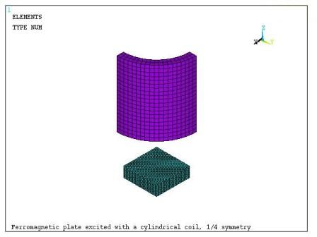
A harmonic electromagnetic analysis is performed to determine the eddy current loss in a ferromagnetic plate. Only a quarter symmetry sector is considered for the analysis (Figure 7.2: Finite Element Model of the Ferromagnetic Plate and Coil). The coil and the plate are enclosed in an air box of size 0.5 x 0.5 x 0.4 m. Flux parallel boundary conditions are imposed on the exterior surface of the air enclosure.
Both the coil and the ferromagnetic plate are modeled using the electromagnetic analysis option (KEYOPT(1) = 1) of SOLID236. In addition, KEYOPT(5) is set to 1 for the coil to suppress the eddy currents. The air box is modeled using the magnetic analysis option KEYOPT(1) = 0.
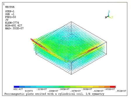
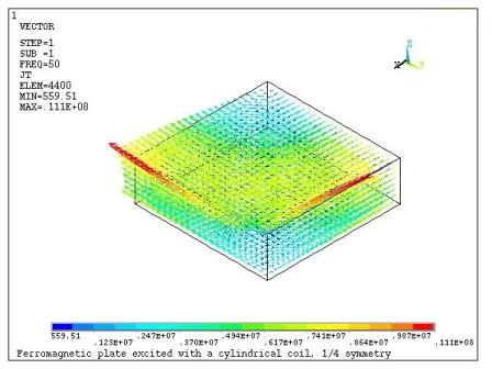
The POWERH command macro is used to calculate the time-averaged (rms) power loss in the plate. Taking into account the symmetry factor, the power loss is found to be Pav=131.9 watts. The real and imaginary components of eddy current density in the plate are shown in Figure 7.3: Eddy Currents Distribution in the Plate (Real Solution) and in Figure 7.4: Eddy Currents Distribution in the Plate (Imaginary Solution), below.
The electromagnetic analysis is followed by a steady-state thermal analysis to determine the temperature distribution in the plate due to Joule heating produced by the eddy currents. The ambient temperature is assumed to be 70 °C. The thermal conductivity and convection coefficient of the plate are taken to be k=50 watts/(m°C) and h=100 W/(m2°C) respectively.
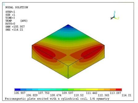
The time-averaged Joule heat generation rate is transferred to the thermal SOLID90 model using the LDREAD,HGEN command. The resulting steady-state temperature distribution is shown in Figure 7.5: Temperature Distribution in the Plate . The average calculated temperature in the plate is Tav=110.1 °C
/title, Ferromagnetic plate excited with a cylindrical coil, 1/4 symmetry
/nopr
/VIEW,1,1,1,1
/VUP,1,Z
/SHOW,win32c     ! use /SHOW,x11c for X Window System
/CONT,1,18

! *** Problem parameters

! Ferromagnetic plate:
lp=0.1           ! length, m
hp=0.015         ! height, m
eszp=0.002       ! element size, m
sigp=6.66e6      ! conductivity, S/m
mu_fer=200       ! relative permeability
k=50             ! thermal conductivity, W/m_C
h=100            ! convection coefficient, W/(m^2_C)

! Coil:
ri=0.05          ! inner radius, m
ro=0.06          ! outer radius, m
hc=0.1           ! height, m
d=0.05           ! distance between the coil and the plate,m
eszc=0.005       ! element  size, m
frq=50           ! frequency, Hz
I=1e5            ! rms coil current, A
mu_coil=1        ! relative permeability

! Air box:
la=0.5           ! length, m
ha1=0.05         ! lower height, m
ha2=0.35         ! upper height, m
esza=0.03        ! element size, m
mu_air=1         ! relative permeability
sigc=2e-8        ! conductivity, S/m
Tamb=70          ! ambient temperature,C

/com,
/com, *** Eddy current analysis
/com,
/PREP7
et,1,236,1       ! AZ-VOLT - ferromagnetic plate
et,2,236,1,,,,1  ! AZ-VOLT (no eddy currents) - coil
et,3,236         ! AZ - air

block,0,lp/2,0,lp/2,0,hp            ! plate
cylinder,ri,ro,hp+d,hp+d+hc,0,90    ! coil
block,0,la/2,0,la/2,-ha1,ha2        ! air
vovlap,all
numcmp,all

mp,murx,1,mu_fer
mp,rsvx,1,1/sigp

mp,murx,2,mu_coil
mp,rsvx,2,sigc

mp,murx,3,mu_air

type,1
mat,1
esize,eszp
vmesh,1

type,2
mat,2
esize,eszc
vmesh,2

msha,1,3D
type,3
mat,3
esize,esza
vmesh,3

asel,s,,,11
nsla,s,1
cp,1,volt,all
f,ndnext(0),amps,I*sqrt(2)  !  rms

asel,s,,,12
nsla,s,1
d,all,volt,0
nsel,all

asel,s,,,3
asel,a,,,5
nsla,s,1
d,all,volt,0
nsel,all

nsel,s,ext
d,all,az,0     ! Flux-parallel magnetic BC
nsel,all
allsel
fini

/SOLU
antyp,harm
harf,,frq
solve
fini

/POST1
set,1,1
esel,s,mat,,1             ! select the plate
POWERH                    ! calculate rms power loss
plve,jt,,,,vect,elem,on   ! plot eddy currents (real part)
set,1,1,,1
plve,jt,,,,vect,elem,on   ! plot eddy currents (imag part)
alls
fini

/com,
/com, Ansys computed power loss = %Pavg*4% watts

/com,
/com, *** Thermal analysis
/com,
/PREP7
ddele,all,az
vsel,s,volu,,1
eslv
et,1,90
LDREAD,hgen
vsel,inve
vclear,all
alls
etdele,2,3

mp,kxx,1,k
nsel,s,ext
sf,all,conv,h,Tamb
nsel,all
fini

/SOLU
anty,static
solve
fini

/POST1
set,1,1
plnsol,temp
nsort,temp
*get,minTemp,sort,,min
*get,maxTemp,sort,,max
avTemp=(minTemp+maxTemp)/2
/com,
/com, Average temperature of the plate = %avTemp% (C)
/com,
fini
This example problem demonstrates the calculation of the magnetic field induced by both the conduction and displacement currents in a parallel plate capacitor filled with a lossy dielectric. Simulation results are compared to the analytical solution.
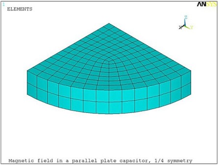
A parallel plate capacitor of radius a = 2 cm and thickness d = 0.5 cm is filled with a lossy dielectric with relative permittivity ε = 3.8 and electrical resistivity ρ = 1000 Ωm. The capacitor is driven by a time-harmonic electric field of magnitude Eo = 2400 V/m at frequency f = 1 MHz. A harmonic electromagnetic analysis is performed to determine the magnetic field induced in the capacitor as a function of distance r from the axis. Only a quarter symmetry sector is considered for the finite element model (Figure 7.6: Finite Element Model of the Lossy Capacitor).
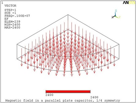
The capacitor is modeled using the electromagnetic analysis option (KEYOPT(1) = 1) of SOLID236. Flux parallel magnetic boundary conditions (AZ = 0) are imposed on the exterior surfaces of the capacitor and on the symmetry planes. The electrodes are defined by coupling the electric potential degree of freedom (VOLT) on the circular surfaces of the capacitor. The electric potential difference Eo*d is applied across the electrodes to create a uniform electric field (Figure 7.7: Electric Field in the Capacitor).
The total current density
induced in the lossy dielectric is composed of the conduction
current density (real part)
and the displacement current density (imaginary part)
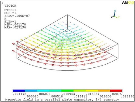
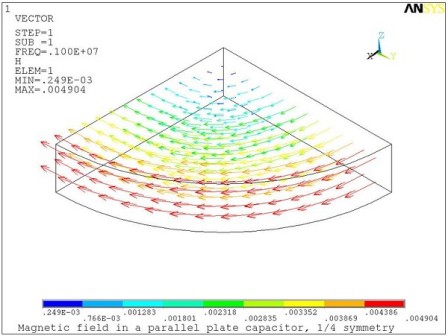
Note that the operating frequency f is low enough to allow neglecting the eddy currents contribution to the conduction current Jc. The conduction and displacement currents induce the real (Figure 7.8: Magnetic Field Induced by the Conduction Current) and imaginary (Figure 7.9: Magnetic Field Induced by the Displacement Current.) magnetic fields, respectively.
Using the Ampere's circuital law:
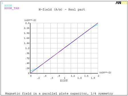
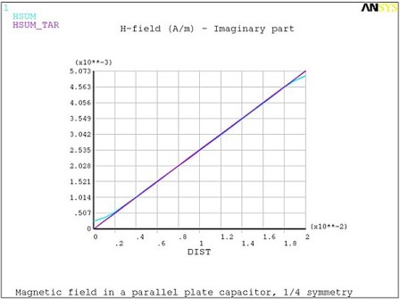
the real and imaginary parts of the magnetic field magnitude can be expressed respectively as follows:
and
These analytical expressions were used to demonstrate the agreement between the Mechanical APDL calculated and the target magnetic field as a function of distance r from the axis. (Figure 7.10: Computed and Analytical Real Magnetic Fields Hr and Figure 7.11: Computed and Analytical Imaginary Magnetic Field Hi )
/title,  Magnetic field in a parallel plate capacitor, 1/4 symmetry
/VIEW,1,1,1,1
/VUP,1,Z
/com,
/com,  Problem parameters:
Pi=acos(-1)
a=2.e-2                        ! radius, m
d=0.5e-2                       ! thickness, m
epsr=3.8                       ! relative permittivity
rho=1000                       ! electrical resistivity, Ohm*m
E=2400                         ! electric field V/m
f=1.e6                         ! frequency, Hz
eps0=8.854e-12                 ! free space permittivity, F/m

Jc=E/rho                       ! conduction current density (Re)
Jd=2*Pi*f*epsr*eps0*E          ! displacement current density (Im)

/nopr
/PREP7
et,1,SOLID236,1                ! AZ+VOLT
mp,perx,1,epsr
mp,rsvx,1,rho
mp,murx,1,1

cyl4,,,,,a,90,d
esize,d/2
vmesh,all

! Electric boundary conditions and loads
nsel,s,loc,z,0
cp,1,volt,all                  ! define bottom electrode
*get,n_grd,node,0,num,min      ! get master node on bottom electrode
nsel,s,loc,z,d
cp,2,volt,all                  ! top electrode
*get,n_load,node,0,num,min     ! get master node on top electrode
nsel,all
d,n_grd,volt,0                 ! ground bottom electrode
d,n_load,volt,E*d              ! apply voltage load to top electrode

! Magnetic boundary conditions for 1/4 symmetry model
nsel,s,loc,z,0
nsel,a,loc,z,d
csys,1
nsel,a,loc,x,a
csys,0
d,all,az,0                     ! flux-parallel BCs
nsel,all
fini

/solu
antype,harm
harfrq,,f
outres,all,all
kbc,1                          ! stepped load
solve
fini

/com,
/com, Compare Mechanical APDL calculated and Expected H-field
/com,
/post1
path,path1,2,10,20
ppath,1,,0,0,0
ppath,2,,0,a,0

/com,
/com, - Real solution
/com,
set,1,1
plvect,ef,,,,vect,elem,on      ! electric field
plvect,jt,,,,vect,elem,on      ! conduction current
plvect,h,,,,vect,elem,on       ! magnetic field

pdef,Hsum,h,sum,avg
pcalc,add,Hsum_tar,s,,Jc/2

/tlabel,-0.2,0.8,H-field (A/m) - Real part
plpath,Hsum,Hsum_tar
prpath,Hsum,Hsum_tar

/com,
/com, - Imaginary solution
/com,
set,1,1,,1
plvect,js,,,,vect,elem,on      ! displacement current
plvect,h,,,,vect,elem,on       ! magnetic field

pdef,Hsum,h,sum,avg
pcalc,add,Hsum_tar,s,,Jd/2

/ann,dele
/tlabel,-0.2,0.8,H-field (A/m) - Imaginary part
plpath,Hsum,Hsum_tar
prpath,Hsum,Hsum_tar

/ann,dele
fini
This example problem demonstrates an harmonic analysis of a transformer.
A transformer consists of primary and secondary coils wound around a ferromagnetic core of high permeability μ. The coils have the same inner and outer radii R1 = 1.5 cm and R2 = 2 cm, respectively, and same height H = 4 cm. The primary coil is characterized by resistance RP = 24 Ω and the number of turns NP. The secondary coil resistance is RS = RP(NS/NP), where NS is the number of turns in the secondary coil. An additional high resistance R = 10000 Ω is attached to the secondary coil to minimize the output current.
The primary coil is energized with an alternating voltage of magnitude V = 1 Volt and frequency f = 50 Hz. The electric current in the primary coil creates a time-harmonic magnetic flux in the core, which induces a voltage in the secondary coil. A harmonic stranded coil analysis is performed to determine the voltage and electromotive force (EMF) induced in the secondary coil. A parametric analysis is also performed to determine how the core permeability μ and the ratio of the number of turns in the coils NS/NP affect the ratio of voltages in the secondary and primary coils.
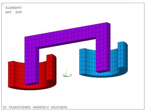
The coils are modeled using the stranded coil option (KEYOPT(1) = 2) of SOLID236. The core and the surrounding air are modeled using the magnetic option (KEYOPT(1) = 0) of SOLID236. The resistance attached to the secondary coil is modeled using the resistor option (KEYOPT(1) = 0) of CIRCU124. Only a quarter symmetry sector is considered for the finite element model (Figure 7.12: Finite Element Model of the Transformer (1/4 Symmetry)). Flux parallel magnetic boundary conditions (AZ = 0) are imposed on the exterior surfaces of the air domain and on the symmetry planes. The VOLT and EMF degrees of freedom are coupled in the coils.
The first harmonic analysis (see the Command Listing) was performed with a core relative permeability μ = 100000 and a coil turn ratio NS/NP = 200. The resulting voltage and EMF in the coils are shown in the following table.
Table 7.2: Coil Voltage and EMF (μ = 100000 and NS/NP = 200)
| Coil | Voltage | EMF |
|---|---|---|
| Primary | 1+j*0 | 0.970+j*0.142 |
| Secondary | -1.919-j*0.281 | -1.937-j*0.284 |
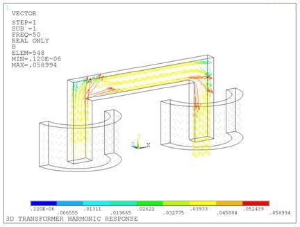
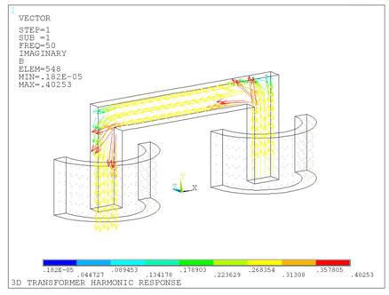
The magnetic flux in the core (real and imaginary) are shown in the following figures.
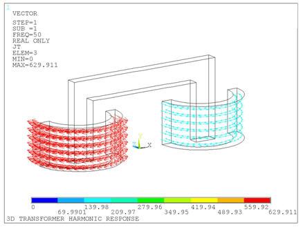
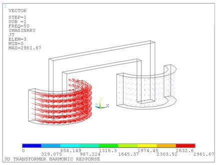
The current density in the primary and secondary coils (real and imaginary) are shown in the following figures.
As shown in the following tables, several subsequent harmonic analyses were performed to study the dependence of the voltage ratio in the coils as a function of core permeability and the ratio of the number of turns.
Table 7.3: Secondary and Primary Coil Voltage Ratio as a Function of Core Permeability μ (NS/NP = 200)
| Core permeability μ | Voltage Ratio VS/VP |
|---|---|
| 1000 | 0.129 |
| 10000 | 1.098 |
| 100000 | 1.94 |
Table 7.4: Secondary and Primary Coil Voltage Ratio as a Function of Ratio of Turns NS/NP (μ = 100000)
| Ration of Turns NS/NP | Voltage Ratio VS/VP |
|---|---|
| 200 | 1.94 |
| 300 | 2.84 |
| 400 | 3.67 |
/title, 3D Transformer Harmonic Response, 1/4 symmetry
/vie,1,2,-1,3
/pnu,mat,1
/num,1
pi=acos(-1)

! *** Model parameters
a_core=0.010        ! core cross-section width
w_core=0.075        ! overall core width
h_core=0.075        ! overall core height

r1_coil=0.015       ! inner radius, both coils
r2_coil=0.020       ! outer radius, both coils
h_coil=0.040        ! height, both coils

d_dmn=0.025         ! depth of surrounding domain

esz1=a_core/3       ! element size, components
esz2=3*esz1         ! element size, surrounding domain

mu_core=100000      ! core permeability


! *** Primary coil
Np=100              ! # of turns
Rp=24               ! DC resistance (ohms)
care_left=(r2_coil-r1_coil)*h_coil      ! cross-sectional area
volu_left=pi*(r2_coil**2-r1_coil**2)*h_coil   ! volume
Vp=1            ! voltage (V)

! *** Secondary coil
Ns=200          ! # of turns
Rs=Rp*(Ns/Np)**2        ! DC resistance (ohms)
care_right=(r2_coil-r1_coil)*h_coil    ! cross-sectional area
volu_right=pi*(r2_coil**2-r1_coil**2)*h_coil   ! volume

R=1e4                   ! resistance attached to the secondary coil

frqncy=50               ! operating frequency (Hz)
symm=4                  ! symmetry factor

/nopr
! *** Geometry
/PREP7
vsel,none               ! core
bloc,-w_core/2,w_core/2,,h_core/2,-a_core/2,0
cm,scrap1_v,volu
vsel,none
bloc,-(w_core/2-a_core),w_core/2-a_core,,h_core/2-a_core,-a_core/2,0
cm,scrap2_v,volu

cmse,s,scrap1_v
cmse,a,scrap2_v
vsbv,scrap1_v,scrap2_v
cm,core_v,volu
vatt,2,2,2

wpcs,-1,0                ! left coil ESYS
wpof,-w_core/2+a_core/2
wpro,,-90
cswp,11,1

wpcs,-1,0                ! right coil ESYS
wpof,w_core/2-a_core/2
wpro,,-90
cswp,12,1

csys

vsel,none                ! left coil
wpcs,-1,11
cyli,r1_coil,r2_coil,0,h_coil/2,0,90
cyli,r1_coil,r2_coil,0,h_coil/2,90,180
vatt,3,3,3,11

vsel,none                ! right coil
wpcs,-1,12
cyli,r1_coil,r2_coil,0,h_coil/2,0,90
cyli,r1_coil,r2_coil,0,h_coil/2,90,180
vatt,4,4,4,12

alls
cm,keep_v,volu
*get,xmin,kp,,mnloc,x
*get,xmax,kp,,mxloc,x
*get,ymax,kp,,mxloc,y
*get,zmin,kp,,mnloc,z

wpcs,-1,0                ! surrounding domain
vsel,none
bloc,xmin-d_dmn,xmax+d_dmn,,ymax+d_dmn,zmin-d_dmn,0
cm,scrap_v,volu

cmse,all
vsbv,scrap_v,keep_v,,dele,keep
cmse,u,keep_v
cm,air_v,volu
vatt,1,1,1

alls
vplo

! *** FE model
et,1,236                 ! air
mp,murx,1,1

et,2,236                 ! core (laminated, non-conducting)
mp,murx,2,mu_core

et,3,236,2               ! left primary coil
mp,murx,3,1
r,3,care_left,Np,volu_left,0,1,0     ! left coil data
rmore,Rp,symm

et,4,236,2               ! right secondary coil
mp,murx,4,1
r,4,care_right,Ns,volu_right,0,1,0   ! right coil data
rmore,Rs,symm

! *** Mesh
numm,kp,1e-8,1e-8
esiz,esz1
vsel,s,mat,,3,4
vmes,all
vsel,s,mat,,2
vswe,all

vsel,s,mat,,1
msha,1
esiz,esz2
vmes,all
alls

! *** Boundary conditions and loads
asel,s,ext             ! flux parallel exterior
csys
asel,u,loc,y
da,all,az

vsel,s,mat,,3          ! left primary coil
alls,belo,volu
cp,1,emf,all
cp,2,volt,all
nd_p=ndnext(0)
alls

vsel,s,mat,,4          ! right secondary coil
alls,belo,volu
cp,3,emf,all
cp,4,volt,all
nd_s=ndnext(0)
alls

d,nd_p,volt,Vp

! *** Circuit
et,5,124,0             ! resistor connected to the secondary coil
r,5,R

*get,nmax,node,,num,max

n,nmax+1,0,h_coil/2
type,5
real,5
e,nd_s,nmax+1

d,nmax+1,volt,0        ! ground
csys

eplo
fini

! *** Solution
/solu
antype,harmonic
harf,frqncy
solve
fini

! *** Post-processing
/post1
set,,,,0               ! Real solution set
Vp_real=volt(nd_p)
Vs_real=volt(nd_s)

/com,
/com, *** Real solution
/com,  Vp = %Vp_real%
/com,  Vs = %Vs_real%
/com,
vsel,s,mat,,2,4
alls,belo,volu
plve,jt,,,,vect,,on
plve,b,,,,vect,,on
plnsol,emf
alls

set,,,,1               ! Imaginary solution set
Vp_imag=volt(nd_p)
Vs_imag=volt(nd_s)

/com,
/com, *** Imag solution
/com,  Vp = %Vp_imag%
/com,  Vs = %Vs_imag%
/com,
vsel,s,mat,,2,4
alls,belo,volu
plve,jt,,,,vect,,on
plve,b,,,,vect,,on
plnsol,emf
alls

Vp = sqrt(Vp_real**2 + Vp_imag**2)
Vs = sqrt(Vs_real**2 + Vs_imag**2)
/com,
/com, *** Secondary to Primary Coil Voltage Ratio =  %Vs/Vp%
fini


