This example shows the nonlinear harmonic analysis of a forced response 1-DOF Duffing oscillator using the harmonic balance method (HBM). Specifically, it demonstrates the following key points:
Definition of a cubic non-linearity using a pre-defined user element (USER300).
Continuation of the solution using the arc-length method.
Direct postprocessing of individual harmonics and manual postprocessing of the total HBM solution.
The example problem is presented in the following sections:
The governing equation of a forced response 1-dof Duffing oscillator is:
(8–1) |
In this example, the parameters of Equation 8–1 are = 1,
= 0.05,
= 1,
= 3, and
= 0.05.
This equation can be modeled using one MASS21 element
linked to a linear spring-damper element (COMBIN14) and a
cubic spring. The cubic spring is modeled using the pre-defined polynomial user
element (USER300, KEYOPT(1) = 2) with real constants RK1 =
and IK1 = 3 for the cubic spring (see the command listing in the next section for details on
the polynomial user element).
The harmonic 1 force is defined using a 2-variable table parameter whose rows depend on the frequency (one value for constant load) and the harmonic index number.
The model is run with 3 harmonics in the frequency range rad/s.
To download the .dat file used for this example problem, click the link below.
The contents of this file are listed below. The command listing shows in detail how to specify and run the HBM analysis. You can use it as a template and modify it to create a custom HBM analysis.
/BATCH,LIST
/TITLE, 1-DOF Oscillator with Cubic Non-linearity
/com =============================================================
/com                    DESCRIPTION:
/com  Harmonic balance analysis for Duffing oscillator's equation:
/com         M*u'' + C*u' + K*u + KNL*u^3 = FEXT*cos(OMG*t)
/com =============================================================

! Model Parameters
PI        = ACOS(-1)
M         = 1         ! MASS
C         = 0.05      ! DAMPING COEFFICIENT
K         = 1         ! LINEAR SPRING CONSTANT
KNL       = 3         ! CUBIC SPRING CONSTANT
FEXT      = 0.05      ! FORCE AMPLITUDE

! HBM and Continuation Parameters
OMGS = 0.60           ! Starting omega
OMGE = 1.50           ! End omega
FMIN = OMGS/(2*PI)    ! Starting frequency
FMAX = OMGE/(2*PI)    ! Ending frequency

DS    = 0.01          ! initial arc length (step length)
DSMIN = DS/50         ! minimum arc length (step length)
DSMAX = 5*DS          ! maximum arc length (step length)

NH    = 3             ! number of harmonics

! __________________ USER_ELEM ____________________
! Internal force
!        Fint = RK0*u   + RK1*u^IK1   + RK2*u^IK2

! UserElem parameters which cannot be modified
NNOD        = 2      ! number of nodes
NDIM        = 3      ! dimension
NNREAL      = 5      ! number of REAL constants
NSAVEVARS   = 0      ! number of saved variables (internal)
NRSLTVAR    = 2      ! number of NMISC items
KEYANSMAT   = 3      ! element characteristics key: non-linear and working in nodal CS

! UserElem parameters to modify
RK0  = 0
RK1  = KNL
IK1  = 3            ! cubic non-linearity
RK2  = 0
IK2  = 0

/PREP7

ET,1,300
KEYOPT,1,1,2       ! polynomial stiffness non-linearity
USRELEM, NNOD, NDIM, LINE, NNREAL, NSAVEVARS, NRSLTVAR, KEYANSMAT
USRDOF,DEFINE, UX
R,1,   RK0, RK1, IK1, RK2, IK2

ET,2,14,0,1        ! linear spring/damper
R,2,K,C

ET,3,21,0,0,4      ! mass
R,3,M

! Geometry
N,1,0,0,0
N,2,1,0,0

TYPE,1
REAL,1
E,1,2

TYPE,2
REAL,2
E,1,2

TYPE,3
REAL,3
E,2

FINISH

/SOLU
ANTYPE,HARMIC

HROPT,HBM,NH                     ! HBM Solve and number of harmonics
HARFRQ,FMIN,FMAX
HBMOPT,CONTSET,,DS,DSMIN,DSMAX   ! Continuation method and step size parameters

! HBMOPT,LIST                    ! List HBM options (optional)
! OUTPR,NSOL,ALL                 ! Print nodal solution (optional)

! Boundary conditions
D,1,ALL
D,2,UY

! Loading
! - Tabular loading definition can be used as a template for harmonic-dependent load.
! - Here, the force is applied to real part of harmonic 1 only and can be
! -                                            directly defined as F,2,FX,FEXT
! - Imaginary loading can also be applied using Value2 on F command:
!     > F,2,FX,,FEXT_IMAG        for imaginary harmonic 1         load
!     > F,2,FX,,%FORCE_TAB_IMAG% for imaginary harmonic-dependent load
!
*dim,FORCETAB,TABLE,1,NH+1,1,FREQ,NHINDEX  ! define table with frequency and harmonic dependency
*DO,HH,0,NH
    FORCETAB(0,HH+1) = HH                  ! COLUMNS: one for each harmonic index
*ENDDO
FORCETAB(1,0) = FMIN                       ! ROWS: one frequency point only for constant loading
FORCETAB(1,2) = FEXT                       ! VALUES: loading for harmonic 1

F,2,FX,%FORCETAB%
KBC,1

SOLVE
FINISH

/COM _________ POST-PROCESSING EACH HARMONIC SOLUTION _________

*get,rstname,ACTIVE,,JOBNAM  ! RST file name

/POST1
FILE,%rstname%_1hi0,rst      ! select result file containing harmonic 1 results
SET,LIST
SET,1,1                      ! print results for 1st frequency point
PRNSOL,U,SUM
FINISH

/POST26
NUMVAR,200
FILE,%rstname%_3hi0,rst      ! select result file containing harmonic 3 results

NSOL ,102,2,u,x              ! store and print frequency history results for harmonic 3
ABS,102,102

/SHOW,png,rev
	/AXLAB,X,Frequency (Hz)
	/AXLAB,Y,Harmonic 3 - amplitude
	PLVAR,102
/SHOW,close
FINISH

/COM _________ POST-PROCESSING CUMULATED HARMONICS SOLUTION _________

postnod       = 2            ! node 		to postprocess
postitem      = 'u'          ! item 		to postprocess
postcomp      = 'x'          ! component to postprocess
ampltype      = 'minmax'

HBM_EXPA,rstname,postnod,postitem,postcomp,NH,ampltype

/com
/com  Pulsation (rad/s)     Amplitude of the response
/com
*VWRITE,_hbm_omg(1),_hbm_ampl(1)
(F16.8,2X,F16.8)

*DIM ,harm_tab   ,table,_Nss,4
*VFUN,harm_tab(1,1),COPY ,_hbm_coeff(1,2)
*VFUN,harm_tab(1,2),COPY ,_hbm_coeff(1,3)
*VFUN,harm_tab(1,3),COPY ,_hbm_coeff(1,6)
*VFUN,harm_tab(1,4),COPY ,_hbm_coeff(1,7)

/SHOW,png,rev
	/AXLAB,X,Pulsation (rad/s)
	/AXLAB,Y,Amplitude
	/GCOLUMN,1,ampl
	*VPLOT,_hbm_omg(1),_hbm_ampl(1)         ! amplitude

	/AXLAB,Y,Harmonic coefficients
	/GCOLUMN,1,h1real
	/GCOLUMN,2,h1imag
	/GCOLUMN,3,h3real
	/GCOLUMN,4,h3imag
	*VPLOT,_hbm_omg(1),harm_tab(1,1),2,3,4  ! harmonic 1 real, 1 imag, 3 real, 3 imag
/SHOW,close
finish

/com
/com  Pulsation (rad/s)     Harmonic 1 real, 1 imag, 3 real, 3 imag
/com
*VWRITE,_hbm_omg(1),harm_tab(1,1),harm_tab(1,2),harm_tab(1,3),harm_tab(1,4)
(F16.8,2X,F16.8,2X,F16.8,2X,F16.8,2X,F16.8)

/exit,nosave
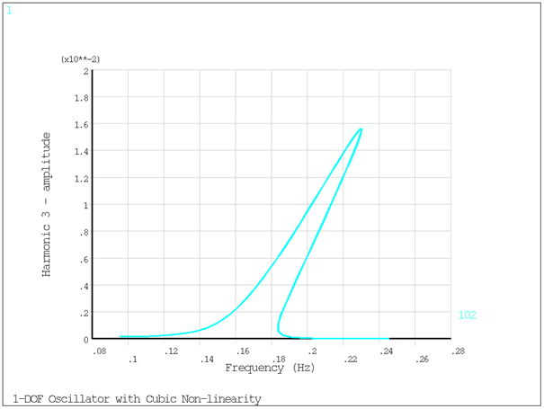
The analysis results are shown below. Direct postprocessing of results for each harmonic can be carried out separately by reading the proper result file (filename_0.rst for harmonic 0, filename_%h%HI0 for harmonic, h) in both /POST1 and /POST26.
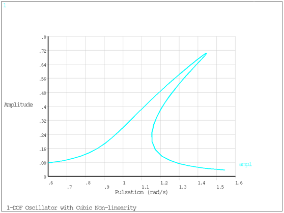
The macro sums all harmonics as described in Appendix A: HBM Macros, and the combined harmonic results are plotted in the following figure.
The resonance frequency of the associated linear model (Equation 8–1 with = 0) is
. The effect of the cubic non-linearity is observed here by a
bending of the response curve toward the right and occurrence of the resonance peak
at a higher frequency (stiffening effect).
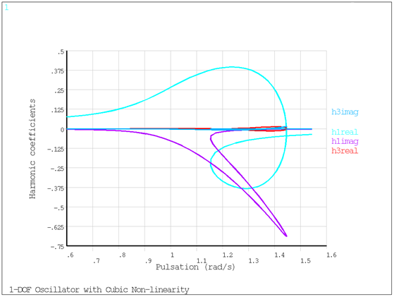
Because of the odd order of the nonlinearity, only odd harmonics contributions are significant (Figure 8.3: Add Harmonic Coefficients harmonics 1 and 3).


