


This section describes the process of creating user defined materials, including the use of the Ansys Additive Material Tuning Tool (Beta) that automates much of the simulation work for you. The following topics are covered:
- 2.1. Overview
- 2.2. Create Material Lookup File (.csv)
- 2.3. Create Material Parameters File (.json)
- 2.4. Run Single Bead Experiments
- 2.5. Identify and Remove Experimental Outliers
- 2.6. Create Experimental Data File (.csv)
- 2.7. Find Characteristic Width Values and Generate Characteristic Width File (.csv)
- 2.8. Find Simulation Parameters to Match Simulation to Experiments
- 2.9. Identify Coefficients for Penetration Depth and Absorptivity
- 2.10. Edit Material Configuration File (.json) and Check Results
- 2.11. User Defined Material File Requirements
Thermal simulations in Additive Science use a simple volumetric heat source model that allows for relatively fast simulations times and is able to accurately capture the size of melt pools associated with additive manufacturing. With this simplified heat source model, the penetration depth and absorptivity are required internal inputs that are generally unknown and vary based on other process parameters. Ansys predefined materials have been established using a material tuning process that determines penetration depth and absorptivity coefficients. With the user defined material capability, you can examine trends and create your own materials that account for these variations in absorptivity and penetration depth.
The penetration depth is defined as the distance a laser heat source can reach down to the material at its 95% cumulative energy. During the additive manufacturing process, the laser can vaporize material in the melt pool, which may sometimes create a vapor cavity within the melt pool. Depending on the laser power level, the vapor cavity size will vary. In general, a larger vapor cavity will contribute to a deeper penetration depth since less energy is lost within the vapor cavity. Our simplified volumetric heat source model does not cover the vapor cavity formation phenomenon, therefore, we need to include coefficients to tune the model with respect to different materials and process parameters.
Four penetration depth coefficients that will be determined by the tuning process are:
penetrationDepthPowderCoeffA
penetrationDepthPowderCoeffB
penetrationDepthSolidCoeffA
penetrationDepthSolidCoeffB
As the laser penetrates into the material, laser reflections and absorption by the vapor cavity affect the fraction of energy absorbed by the melt pool. The fraction of energy absorbed by the melt pool is defined as absorptivity. Since our model simplifies the laser interactions with the vapor, we need to include coefficients to tune the model with respect to different materials and process parameters.
Four absorptivity coefficients that will be determined by the tuning process are:
absorptivityPowderCoeffA
absorptivityPowderCoeffB
absorptivitySolidCoeffA
absorptivitySolidCoeffB
Ansys Additive Science relies on temperature dependent thermal properties for its simulations. These properties can be identified through experiments, literature, or CALPHAD software. For best results, we recommend using material properties of additively manufactured materials, specifically.
The required temperature dependent properties are as follows and their values should be provided for a temperature range from 2 Kelvin to 15000 Kelvin in intervals of 2 Kelvin:
Thermal Conductivity (W/m/K)
Specific Heat (J/kg/K)
Density (kg/m3)
Thermal Conductivity Ratio: Ratio of powder conductivity to solid conductivity. Typically, we use the following values with respect to different temperature ranges:
Thermal Conductivity Ratio = 0.01 when temperature is from 2K to 0.6 times the solidus temperature of the material
Thermal Conductivity Ratio = 0.4 when temperature is from 0.6 times the solidus temperature to the liquidus temperature of the material
Thermal Conductivity Ratio = 1 when temperature is from the liquidus temperature and above
Density Ratio: Ratio of powder density to solid density. Typically, we use the following values with respect to different temperature ranges:
Density Ratio = 0.6 when temperature is from 2 K to the liquidus temperature of the material
Density Ratio = 1 when temperature is from the liquidus temperature and above
Specific Heat Ratio: Ratio of powder specific heat to solid specific heat. Typically, 1.
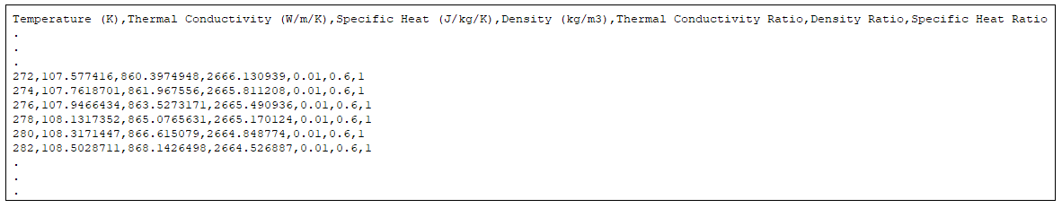
The temperature dependent properties should be organized into a .csv material lookup file with columns of Temperature (Kelvin), Thermal Conductivity (W/m/K), Specific Heat (J/kg/K), Density(kg/m3), Thermal Conductivity Ratio, Density Ratio and Specific Heat Ratio.
Important: Our tuning tool can read only “,” format so take care if you are from regions with different localization settings. Be sure to use “,” instead of “;” in your .csv file.
A portion of the table is shown below. Temperatures are represented as integers from 2K to 15000K, in intervals of 2K. For more information, refer to Material Lookup Table.
| Temperature (K) | Thermal Conductivity (W/m/K) | Specific Heat (J/kg/K) | Density (kg/m3) | Thermal Conductivity Ratio | Density Ratio | Specific Heat Ratio |
| 272 | 5.98 | 536.42 | 4348.75 | 0.01 | 0.6 | 1 |
| 274 | 6.02 | 536.59 | 4348.75 | 0.01 | 0.6 | 1 |
| 276 | 6.05 | 537.48 | 4348.75 | 0.01 | 0.6 | 1 |
| 278 | 6.08 | 538.89 | 4348.75 | 0.01 | 0.6 | 1 |
| 280 | 6.11 | 540.18 | 4348.75 | 0.01 | 0.6 | 1 |
| 282 | 6.14 | 541.24 | 4348.75 | 0.01 | 0.6 | 1 |
Here is the .csv file for the example table above.
Besides the six temperature dependent thermal properties described in the previous section, you will also need to obtain a set of material properties and model coefficients for the model tuning process.
The following figure shows an AlSi10Mg material parameters file example. It stores three categories of parameters: material inherent properties, material mechanical properties and model tuning coefficients. Four penetration depth tuning coefficients and four absorptivity tuning coefficients are included in the model tuning coefficients category and are all set to 0 as the beginning of the tuning process. You need to obtain all parameter values and store them in the layout shown in .json format.
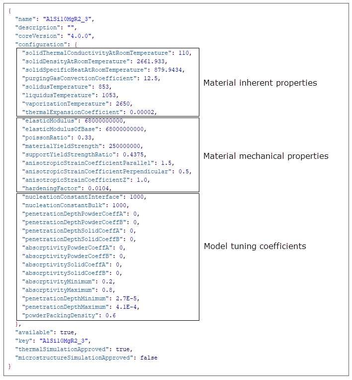
For details and default values of parameters in the material parameters file, refer to Material Configuration File.
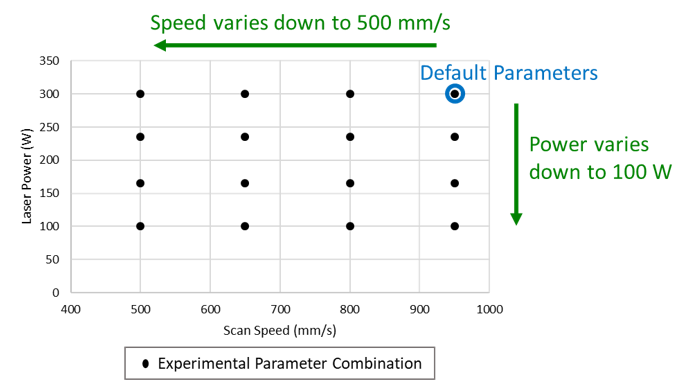
To tune the volumetric heat source model for a user defined material, you need to run a series of single bead experiments to compare with simulation results. At a minimum, 9 different parameter combinations should be used. To identify what parameter combinations to use, a good method is to base them on default parameters for the alloy of choice or an alloy with similar thermal properties. The default parameter set is defined as the machine vendor recommended process parameter set or the material manufacturer's optimized process parameter set. Use this parameter combination as the high power-high speed case and vary power and speed lower from there. Generally, 100W and 500 mm/s are decent choices for lower power and speed thresholds. Space out a grid of parameter combinations between the high and low bounds for speed and power, and use this grid as a basis for the experiments. You may want to remove some of the low power-high speed cases as the melt pools may be inconsistent and difficult to measure in those areas. An example of a range of experimental parameters is shown in the following figure.
We recommend you build the single beads on pads with a layer of powder added. This ensures that the experimental conditions more closely match the conditions you will find in a build when considering material properties and powder layer thickness. Make sure to use default process parameters for pad fabrication to achieve the best top surface layer quality possible. The following are some additional suggestions for experiments:
Make at least 3 replications for single bead at each P-V combination.
Each single bead scan should be at least 10 mm long.
Scan single beads perpendicular to the final layer of the as-built pad to create contrast.
Keep laser beam diameter and preheat temperature constant for all experiments.
Allow time to cool down to the preheat temperature after the spread of the powder layer to minimize the shrinkage effect of the as-built substrate before depositing the single beads.
Sample the melt pool cross sections near the middle point of each single bead scan to ensure a stable scanning condition.
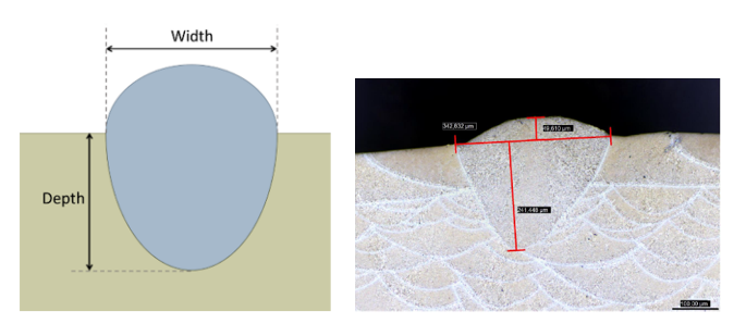
After the single bead samples have been fabricated, they should be sectioned, polished, etched, and then measured for melt pool cross-sectional dimensions. Measurements should be taken from multiple cross sections or multiple samples of each parameter set for more consistent results. Melt pool width and depth should be measured from the substrate surface as shown in the following figure. These melt pool experimental dimensions correspond to the median reference melt pool dimensions in the simulation.
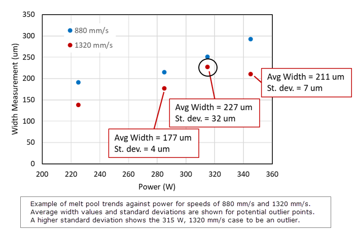
After single bead widths and depths have been measured, it is time to check for outliers in the experimental dataset. First, review the trends in the measurements to check for any unexpected changes in depth or width. For instance, melt pool size should be expected to decrease with an increase in speed for a fixed power. Similarly, melt pool size should be expected to decrease with a decrease in power for a fixed speed. If certain points in your dataset do not follow the expected trends, these experimental data points should be omitted or remeasured. To determine which point or points are outliers, you can compare the deviation of measurements from different locations along the single bead, or look at the quality of individual melt pools.
The following figure shows an example where melt pool widths at 880 mm/s follow an acceptable trend with power, but widths at 1320 mm/s show a decrease when going from 315 to 345 W. Taking a look at the data from the cases near the problematic parameter combinations, we can see a significantly higher standard deviation for the 315 W, 1320 mm/s case. This parameter combination is an outlier and cross sections should be remeasured, or the case should just be omitted from future use.
In some cases, low quality or balling single beads can make it difficult to get consistent measurements. If single bead melt pools look to be exhibiting balling or other issues but full parts or porosity samples show low porosity, the single bead experiments can be modified to show more consistent results. To do this, deposit multiple scan lines next to each other in a single layer pad. This can create more consistent melt pool sizes and enable better measurements of melt pool depth and width. If you use this strategy, repeat it for all parameter combinations to ensure consistency.
In cases where melt pool morphologies are not distinguishable from the as-built pad microstructures (e.g., Ti64), depositing a layer of powder directly onto a wrought or cast plate of the same material for the single bead experiments is an option. However, in this case, the layer thickness value that you specify in the experimental data file should be equal to the actual powder layer thickness used in the experiments multiplied by the powder packing density. For example, if a 60 µm layer thickness of powder is deposited onto the plate and the powder packing density is 0.6, then the actual layer thickness that you should use in the experimental data file is 60*0.6=36 µm. This is because the simulation uses the layer thickness after solidification instead of the actual powder layer thickness.
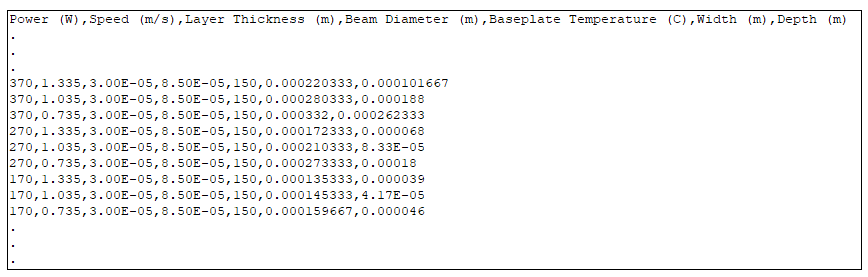
After the appropriate experimental dataset has been identified, arrange the data as shown in the following table. (This example shows only a portion of the data.) Then create the experimental data .csv file. Make sure to use the exact header and units as shown.
Important: Our tuning tool can read only “,” format so take care if you are from regions with different localization settings. Be sure to use “,” instead of “;” in your .csv file.
| Power (W) | Speed (m/s) | Layer Thickness (m) | Beam Diameter (m) | Baseplate Temperature (C) | Width (m) | Depth (m) |
| 370 | 1.335 | 3.00E-05 | 8.50E-05 | 150 | 0.000220333 | 0.000101667 |
| 370 | 1.035 | 3.00E-05 | 8.50E-05 | 150 | 0.000280333 | 0.000188 |
| 370 | 0.735 | 3.00E-05 | 8.50E-05 | 150 | 0.000332 | 0.000262333 |
| 270 | 1.335 | 3.00E-05 | 8.50E-05 | 150 | 0.000172333 | 0.000068 |
| 270 | 1.035 | 3.00E-05 | 8.50E-05 | 150 | 0.000210333 | 0.0000833 |
| 270 | 0.735 | 3.00E-05 | 8.50E-05 | 150 | 0.000273333 | 0.00018 |
| 170 | 1.335 | 3.00E-05 | 8.50E-05 | 150 | 0.000135333 | 0.000039 |
| 170 | 1.035 | 3.00E-05 | 8.50E-05 | 150 | 0.000145333 | 0.0000417 |
| 170 | 0.735 | 3.00E-05 | 8.50E-05 | 150 | 0.000159667 | 0.000046 |
Here is the .csv file for the example table above.
The characteristic widths are simulation melt pool widths from single bead simulations with no powder and a very small surface heat source. It serves as a reference benchmark for the melt pool width created by a point source laser. The characteristic width file is required to create a user defined material in the Materials Library. Absorptivity in these cases should be close to the low end of the values found in the previous step; generally, this will be around 0.2.
Keep the baseplate temperature the same as the one in the single bead experiments to generate the characteristic width file. Create a characteristic width lookup table and interpolate to find characteristic widths for each experimental parameter combination. You can run simulations across the provided set of power-speed combinations for characteristic widths. Once you have a characteristic width from each combination, create a characteristic width .csv file with columns of power (W), speed (m/s), and characteristic width (m). The Material Tuning Tool automates the simulations and interpolation for you.
When using the Material Tuning Tool, 8 levels of laser power and 8 levels of scan speed are used as defaults to create 64 combinations for the characteristic width file generation.
Laser power (W): 50, 100, 150, 200, 300, 400, 500, 700
Scan speed (mm/s): 350, 500, 750, 1000, 1250, 1500, 2000, 2500
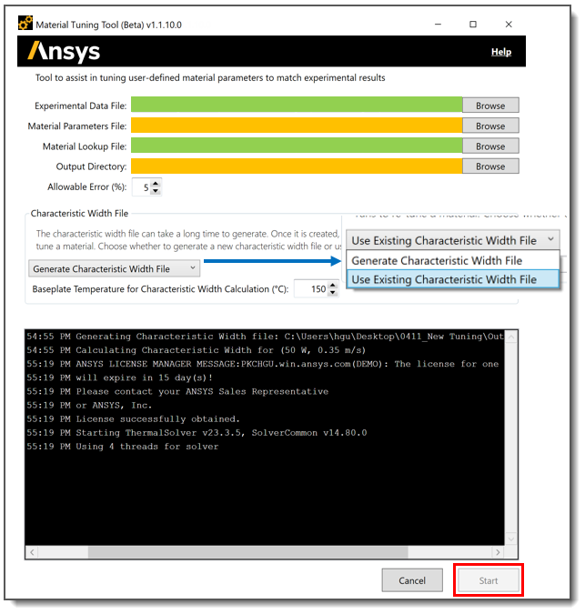
Choose to either upload an existing characteristic width table or generate a new one in the Material Tuning Tool.
For details and default values of parameters in the Characteristic Width File, refer to Characteristic Width Lookup Table.
Once experimental data has been gathered, you need to find the model parameters that result in matching simulation and experimental melt pool dimensions. The two unknown parameter sets that must be determined for the model are the absorptivity and heat source penetration depth. Both values will vary based on the process parameters used. In higher energy density scenarios, the laser vaporizes material in the melt pool and penetrates into the substrate. As the penetration depth increases, the fraction of energy absorbed by the melt pool increases due to internal reflections and other effects.
For each parameter combination, you will need to iterate to find matching absorptivity and penetration depth values. To start, you may want to choose a penetration depth that is near the experimental melt pool depth, and an absorptivity around 0.5. Once you have simulation results from an iteration, compare them to experimental results and adjust the absorptivity and penetration depth to step closer to experimental results. In general, increasing absorptivity will increase both the melt pool width and depth. Increasing penetration depth will increase melt pool depth and can slightly affect melt pool width. In the Ansys Additive Material Tuning Tool, we set the starting penetration depth and absorptivity values as fixed, at 0.0001 m and 0.5 respectively.
Iterate on each parameter combination until experimental and simulation results are within an acceptable error tolerance (5% suggested). Once this has been achieved, record the model inputs used to create the results and move on to the next parameter set. Repeat this process until you have absorptivity and penetration depth parameters for each experimental case.
In some cases, you may not be able to find an absorptivity and penetration depth combination that results in melt pool dimensions within the given tolerances. In these cases, mark the parameter combination as unconverged and continue to the next parameter set. If this happens across many cases, you may want to check some of the other parameter inputs such as beam diameter to see if there are errors in the input values.
The Material Tuning Tool automates the above-mentioned iteration process and caps the number of iterations at 15. To start the automatic tuning process, import the above mentioned three files, experimental data file, material parameters file and material lookup file. Then specify an output directory and allowable error percentage. Choose either uploading an existing characteristic width table or generating a new one in the Material Tuning Tool. Once everything is configured, click the Start button to run the automatic tuning process. Note that when running the Material Tuning Tool, you can still run Additive Print and Science simulations.
Once the Material Tuning Tool is completed, a .csv file called Optimized_Parameters will be created in the output folder. This Optimized_Parameters file contains information that will be used to determine penetration depth and absorptivity coefficients.
If you chose to generate the characteristic width file, a CW_Lookup .csv file will also be created in the output folder.
Using the Optimized_Parameters file, obtain penetration depth and absorptivity coefficients via simple linear regression.
The following figure shows a portion of an Optimized_Parameters file.
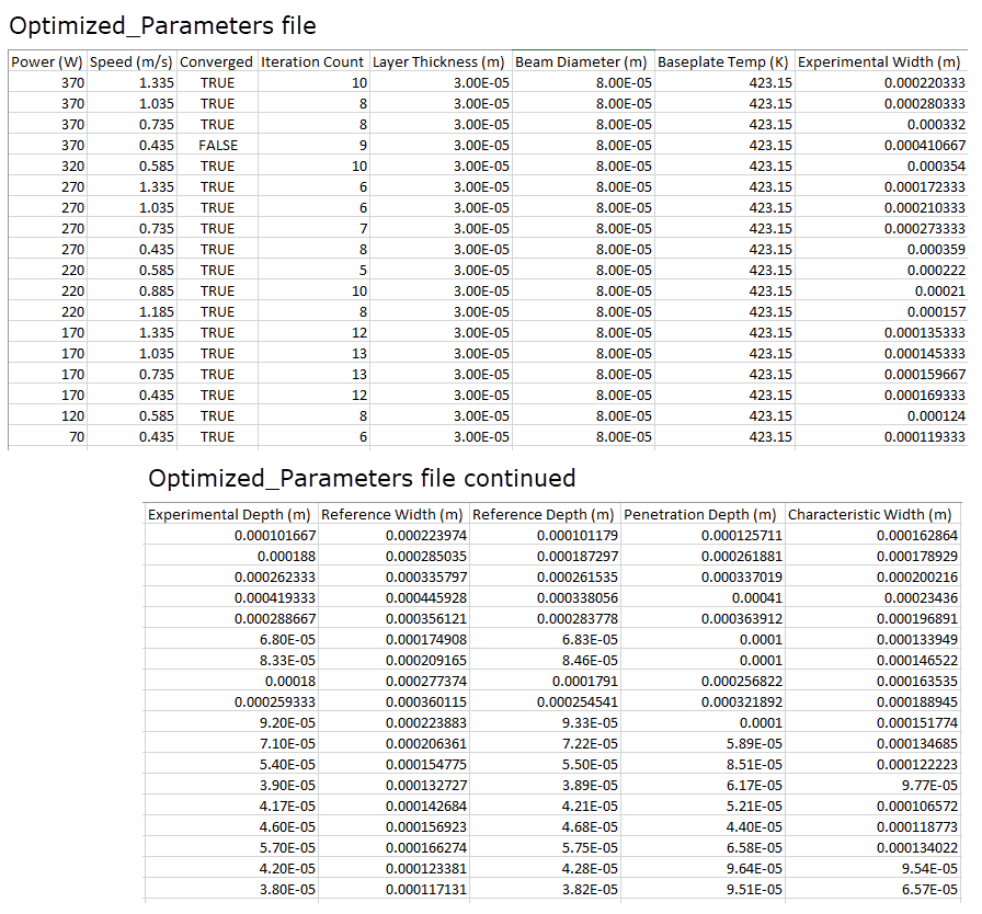
First, filter out FALSE rows in the Converged column. This will remove all unconverged parameter combinations. (Unconverged means the simulation melt pool reference dimensions did not reach the experimental melt pool dimensions within the provided error tolerance.)
Next, focus on the last 3 columns of the file.
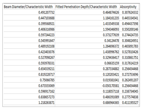
The Fitted Penetration Depth is defined as following:

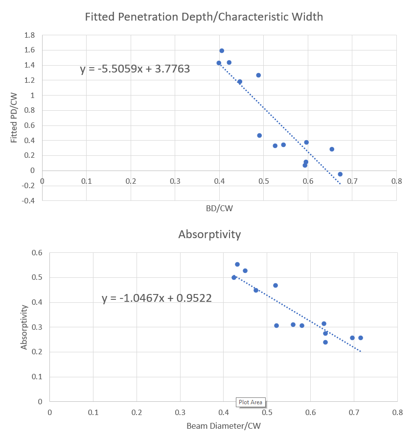
Plot Fitted Penetration Depth/Characteristic Width against Beam Diameter/Characteristic Width. Graph a line-of-best-fit on the data in the format shown below:

A is the penetrationDepthPowderCoeffA and penetrationDepthSolidCoeffA in your material configuration file (.json).
B is the penetrationDepthPowderCoeffB and penetrationDepthSolidCoeffB in your material configuration file (.json).
To get the penetration depth coefficients, plot Absorptivity against Beam Diameter/Characteristic Width. Remove data points that are outliers of a linear trend where the absorptivity already hits the bound. Again, graph a line-of-best-fit on the data in the format shown below:

Here, A is the absorptivityPowderCoeffA and absorptivitySolidCoeffA to be used in your material configuration file (.json).
Here, B in the absorptivityPowderCoeffB and absorptivitySolidCoeffB to be used in your material configuration file (.json).
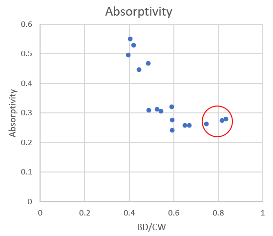
In addition, the upper and lower limits for penetration depth and absorptivity are defined using penetrationDepthMaximum, penetrationDepthMinimum, absorptivityMaximum and absorptivityMinimum in the material parameters file. When you start to notice that fitted PD/CW and/or absorptivity values stabilize with the change of BD/CW, as in the above two plots, adjust penetrationDepthMaximum, penetrationDepthMinimum, absorptivityMaximum and absorptivityMinimum to avoid those regions. For example, when BD/CW changes from 0.7 to 0.85 in the following plot, the absorptivity does not change much. It is very likely that the absorptivity for these cases already reached the lower limit. You can lift up the lower limit of absorptivity by increasing the absorptivityMinimum value to a higher one for another tuning.
Using the coefficients found in the previous step, fill out the appropriate fields in your material parameters file as shown in the following table. Save the file as your Material Configuration File (.json).
| penetrationDepthPowderCoeffA | A from modified penetration depth best fit line |
| penetrationDepthPowderCoeffB | B from modified penetration depth best fit line |
| penetrationDepthSolidCoeffA | A from modified penetration depth best fit line |
| penetrationDepthSolidCoeffB | B from modified penetration depth best fit line |
| absorptivityPowderCoeffA | A from absorptivity best fit line |
| absorptivityPowderCoeffB | B from absorptivity best fit line |
| absorptivitySolidCoeffA | A from absorptivity best fit line |
| absorptivitySolidCoeffB | B from absorptivity best fit line |
| absorptivityMinimum | 0.2 [a] |
| absorptivityMaximum | 0.8 [a] |
| penetrationDepthMinimum | 2.7E-5 [a] |
| penetrationDepthMaximum | 4.1E-4 [a] |
[a] Recommended value
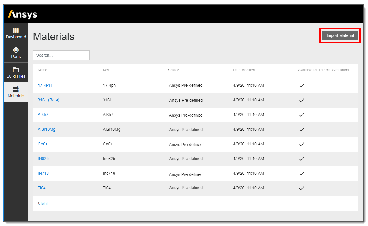
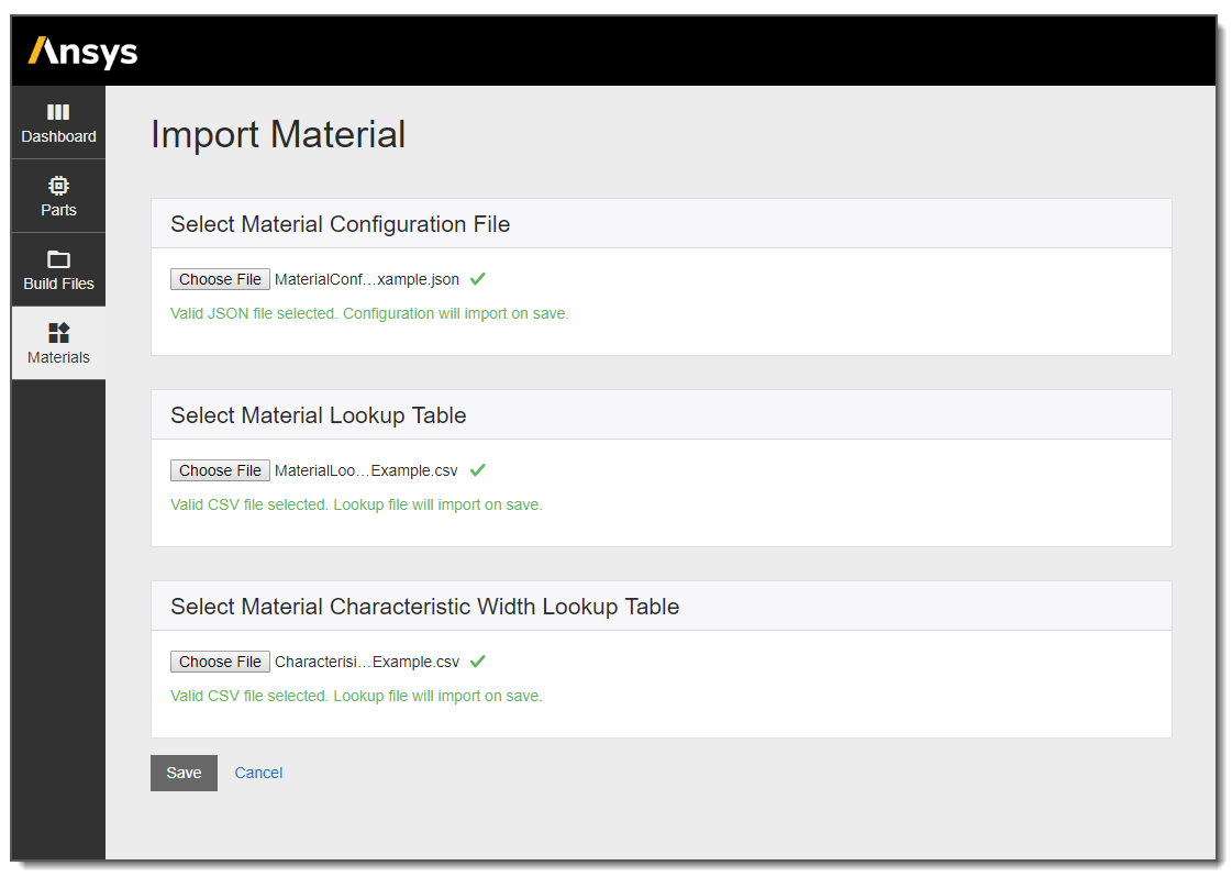
To add a user defined material to the Additive application for future use, open the Materials Library and click Import Material.
Navigate to upload the three appropriate files and click Save.
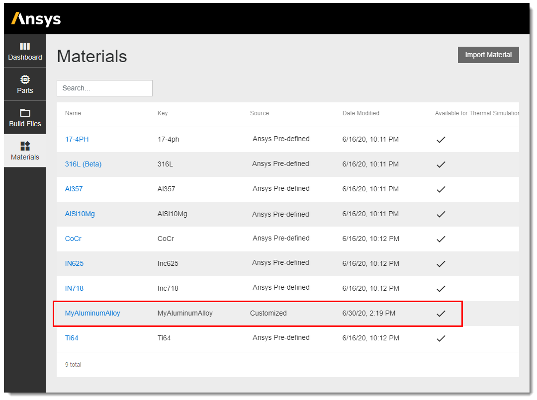
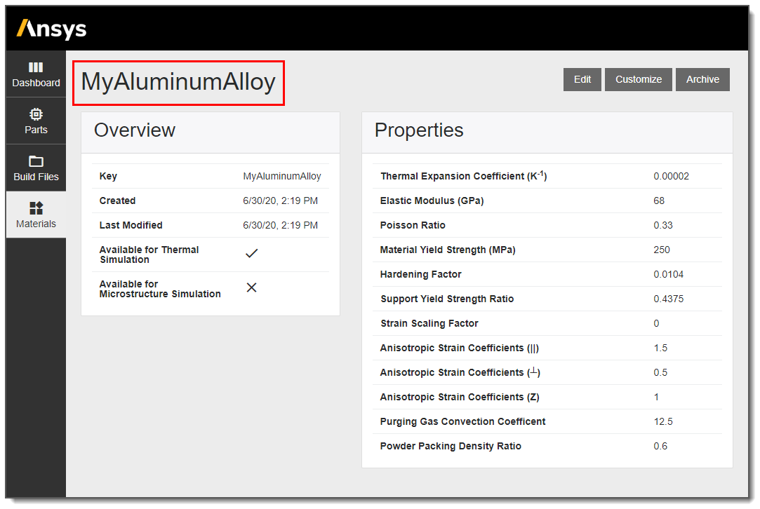
Now when you view the Materials Library listing, you will see your new user defined material. Click on it to see details.
Run a few cases from your experimental set to evaluate the accuracy of the inputs before continuing to use the settings throughout the product.
Use the Archive button to remove the user defined material from the Materials Library. Simulations using this material will remain.
Overview
The material configuration file contains information on mechanical properties, constant thermal properties, and other parameters used in Additive Science. This file is read as part of the input when running any simulation, but not every setting is used in every simulation.
Settings defined in the material configuration file are defined below:
| Setting | Definition | Units | Value |
| name | Name for the material. Must be unique. | - | |
| description | Additional comments (optional) | - | |
| coreVersion | Version of the current material configuration file. This can be changed when updating new versions of the same material. | - | |
| solidThermalConductivityAtRoomTemperature | Thermal conductivity of bulk material at room temperature (298 K) | W/m/K | |
| solidDensityAtRoomTemperature | Density of bulk material at room temperature (298 K) | kg/m^3 | |
| solidSpecificHeatAtRoomTemperature | Specific heat of bulk material at room temperature (298 K) | J/kg/K | |
| purgingGasConvectionCoefficient | Convection coefficient between the solid and gas during processing | W/(m^2*K) | 12.5 |
| solidusTemperature | Maximum temperature at which the material is completely solid | K | |
| liquidusTemperature | Minimum temperature at which the material is completely liquid | K | |
| vaporizationTemperature | Temperature at which material has completely changed from liquid to vapor | K | |
| thermalExpansionCoefficient | Coefficient of thermal expansion. | 1/K | |
| elasticModulus | Elastic modulus of build material. | Pa | |
| elasticModulusOfBase | Elastic modulus of base material. | Pa | |
| poissonRatio | Poisson ratio | - | |
| materialYieldStrength | Yield strength | Pa | |
| supportYieldStrengthRatio | Factor to reduce the yield strength and elastic modulus of support material | - | |
| anisotropicStrainCoefficientParallel | Multiplier on the predicted strain in the direction that the laser is scanning for the major fill rasters | - | 1.5 |
| anisotropicStrainCoefficientPerpendicular | Multiplier on the predicted strain orthogonal to the direction that the laser is scanning for the major fill rasters and in the plane of the surface of the build plate | - | 0.5 |
| anisotropicStrainCoefficientZ | Multiplier on the predicted strain in the Z direction | - | 1 |
| hardeningFactor | Factor relating the elastic modulus to the tangent modulus for plasticity simulations (Tangent Modulus = elasticModulus*hardeningFactor ) | - | |
| nucleationConstantInterface | Controls the heterogeneous nucleation rate (on existing solid interfaces) during solidification for the microstructure solver | 1/m/K^2 | 1000 |
| nucleationConstantBulk | Controls the homogenous nucleation rate (in bulk of the microstructure simulation domain) during solidification for the microstructure solver | 1/m^2/K^2 | 1000 |
| penetrationDepthPowderCoeffA | Coefficients used in thermal analyses to control absorptivity and penetration depth. These settings are determined through tuning. | - | |
| penetrationDepthPowderCoeffB | |||
| penetrationDepthSolidCoeffA | |||
| penetrationDepthSolidCoeffB | |||
| absorptivityPowderCoeffA | |||
| absorptivityPowderCoeffB | |||
| absorptivitySolidCoeffA | |||
| absorptivitySolidCoeffB | |||
| absorptivityMinimum | Minimum fraction of energy absorbed by the melt pool (for example, 0.2 means 20%) | Dimensionless fraction | 0.2 [a] |
| absorptivityMaximum | Maximum fraction of energy absorbed by the melt pool (for example, 0.8 means 80%) | Dimensionless fraction | 0.8 [a] |
| penetrationDepthMinimum | Lower limit for penetration depth | m | 2.7E-5 [a] |
| penetrationDepthMaximum | Upper limit for penetration depth | m | 4.1E-4 [a] |
| powderPackingDensity | Density of powder material relative to the solid | Dimensionless fraction | 0.6 [a] |
| available | True | ||
| key | Unique name for the material. Must be 16 characters or fewer, contain no spaces, and can be the same as the "name." | - | |
| thermalSimulationApproved | True or false flag signifying whether the material can be used for thermal simulations. | - | True |
| microstructureSimulationApproved | True or false flag signifying whether the material can be used for microstructure simulations. | - | False |
[a] Recommended value
Format
These inputs are laid out in a .json file format with material properties held within the configuration parameter. An example of this file is provided as MaterialConfigurationExample.json. When editing values from the example or creating your own material configuration file, be sure to follow the json format to avoid errors.
Overview
The material lookup table contains temperature dependent thermal properties for the material. This data is required by the Thermal Solver used in Additive Science simulations as well as the Thermal Strain simulation type in Additive Print.
The temperature dependent properties consist of thermal conductivity, specific heat, and density for an additive manufacturing material. In addition to properties for solid and liquid material, properties for the powder state are specified through ratios for each property. For example, if the density of the powder material is half that of the solid, a value of 0.5 would be provided for the Density Ratio.
Format
The material lookup file is a .csv file with seven columns representing Temperature (K), Thermal Conductivity (W/m/K), Specific Heat (J/kg/K), Density (kg/m^3), Thermal Conductivity Ratio, Density Ratio, and Specific Heat Ratio. An example of this file is provided as MaterialLookupExample.csv.
Temperature: At a minimum, points at the transition temperatures (solidus, liquidus, and vaporization) must be provided. The transition temperatures must be within ±1K of those provided in the material configuration file. An interpolation function will calculate the remaining points on the property curves from 2K to 15000K. The code is designed to fetch an additional input corresponding to the room temperature properties (solidThermalConductivityAtRoomTemperature, solidDensityAtRoomTemperature, solidSpecificHeatAtRoomTemperature) from the material configuration file for the interpolation. This information may or may not be in the material lookup table. Adding additional points in the material lookup table besides at the transition temperatures will contribute to the accuracy of the interpolation.
Note: A full-length lookup file with temperatures from 2K to 15000K defined in intervals of 2K was required previous to release 2024 R1. If this is provided, the code skips the interpolation function.
Thermal Conductivity Ratio values should be as follows:
Ratio = 0.01 from 2K to 0.6 x the solidus temperature of the material
Ratio = 0.4 from 0.6 x the solidus temperature to the liquidus temperature of the material
Ratio = 1 from the liquidus temperature to 15000K.
Density Ratio values should be as follows:
Ratio = 0.6 from 2K to the liquidus temperature of the material. (0.6 is a recommended value. It must correspond to powderPackingDensity in the material configuration file.)
Ratio = 1 from the liquidus temperature to 15000K.
Specific Heat Ratio should be 1.
Overview
The characteristic width lookup table is used to find characteristic widths for different parameter combinations. This table is generated as part of the single bead tuning process and will be used to help determine heat source penetration depth and absorptivity for all thermal simulations. The table contains data points for characteristic width at different power and speed combinations.
Format
The characteristic width lookup table is in .csv format with columns for speed (m/s), power (W), and characteristic width (m). Speeds and powers in the first two columns should span the range of possible inputs for those two parameters. The power-speed combinations should be organized such that there is a characteristic width value for each power at each speed, creating a rectilinear grid. An example of this file is provided as CharacterisiticWidthExample.csv.