For any simulation in Mechanical, once a solution is available you can view a contour plot or animate the results. There are solutions at many time points in a transient analysis and you can display the variation of a result item at a location over time. So for a LPBF Thermal-Structural simulation you can view a result at a location on the build over the build history.
In addition to those general results, the following are result items of particular concern for AM simulations:
Recoater Interference – The LPBF Recoater Interference result tool allows you to identify excessive deformation in the Z direction that may lead to interference with the powder spreading mechanism during printing.
High Strain – The LPBF High Strain result tool allows you to identify regions of the part that may be prone to forming cracks during or after the build process by highlighting critical strain values.
Hotspot – The LPBF Hotspot result tool is used to identify areas of overheating that may result in problematic thermal conditions. This result is available for thermal-structural simulations only.
Deformation Along a Line – At times you may want to obtain results along an edge or other specific location of the part to determine if the part will be within tolerances or to compare to distortion measurements made after the part is built. This technique is used when calibrating Strain Scaling Factors, for instance. There are several ways to obtain this result.
3D Printing Time Estimate – Get an estimate of the real 3D printing time.
Procedural Steps
Recall that you used Output Controls under Analysis Options and/or AM-specific result items to control which items are solved for in the simulation. Perhaps you set up results trackers in the solution step to observe the results being processed during the solution. When reviewing results after the solution, you will generally need to evaluate results to obtain them for viewing. Evaluating results is a way to retrieve them from the data that was stored during solution. Only data items that were solved for may be retrieved in this way.
There are many different ways to view results but some of the ones most commonly used for additive manufacturing are described here:
Animate Thermal Results - Temperatures (Thermal-Structural System)
In the project tree under Transient Thermal, select the Solution object and then, in the context menu, click Thermal and then Temperature. Or right-click Insert > Thermal > Temperature. A Temperature object is created and becomes active.
Right-click Temperature and select Evaluate All Results. This retrieves the temperature data and displays it in both graph and tabular form.
Use the animation controls at the top of the Graph window. Click the Result Sets button
 and also the Update
Contour Range at Each Animation Frame button
and also the Update
Contour Range at Each Animation Frame button  . Adjust the number of seconds for the animation
and click Play. For more information about animation
controls, see Animation in the Mechanical User's Guide.
. Adjust the number of seconds for the animation
and click Play. For more information about animation
controls, see Animation in the Mechanical User's Guide.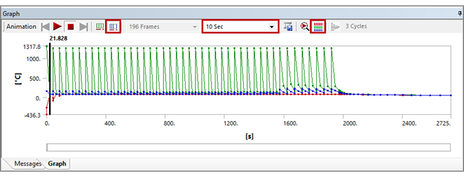
The following is an animated GIF. Refresh the page to see the animation. View online if you are reading the PDF version of the help.
Animate Structural Results - Total Deformation
In the project tree under Static Structural, select the Solution object and then, in the context menu, click Deformation and then Total. A Total Deformation object is created and becomes active.
Right-click Total Deformation and select Evaluate All Results. This retrieves the deformation data and displays it in both graph and tabular form.
Use the animation controls at the top of the Graph window.
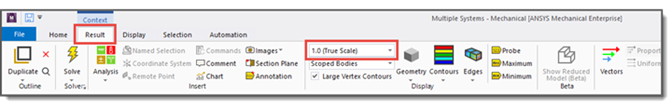
It is important (and fun!) to change the magnification scale of the display in the Geometry window so you can get a true sense (or an exaggerated sense) of the deformation in your build. With Total Deformation highlighted in the project tree, from the Result context tab, select the True Scale option from the drop-down menu. Animate the results using the animation controls. Select other scales from the drop-down menu to see exaggerated results.
The following is an animated GIF. Refresh the page to see the animation. View online if you are reading the PDF version of the help.
Check for Recoater Interference
You need to define some sort of threshold for the level of Z-deformation that is considered to be recoater interference. In the LPBF Recoater Interference Details view, change the Threshold Definition to one of these three options:
None - The result tool will show pure Z-deformation in the build, where the value at each point corresponds to the Z-deformation when that material was a new layer.
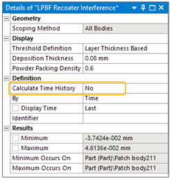
Layer Thickness Based (default) - The result tool uses the Deposition Thickness (set in the Build Settings object for some simulation types, otherwise set it here) and a new input field, Powder Packing Density, to determine the thresholds for warning and critical deformation. Specifically, if the Z-deformation for any layer is equal to or greater than the Deposition Thickness it is considered a warning. If the Z-deformation is equal to or exceeds the value of Deposition Thickness/Powder Packing Density, it is considered critical. Powder Packing Density may be dependent on the powder particle size, material, spreading mechanism, or other factors.
User Defined - You define your own warning and critical thresholds.
Once you have chosen your Threshold Definition, right-click the LPBF Recoater Interference object and select Evaluate All Results. The resulting display shows the model with absolute Z-deformation values but with color contours based on the threshold criteria you selected. For the Layer Thickness Based and User Defined options, contours are shown as follows:
Blue = Safe (Layer Thickness Based: Z-deformation is less than Deposition Thickness)
Green = Warning (Layer Thickness Based: Z-deformation is equal to or greater than the Deposition Thickness)
Red = Critical (Layer Thickness Based: Z-deformation is equal to or exceeds the value of Deposition Thickness/Powder Packing Density)
Important: The data displayed is based on the Z deformation of each layer right before the next layer is added. It does not represent the "final state" of deformation at the end of the cooldown step.
Note: To ensure a quick, dynamic calculation of results, Calculate Time History is set to No by default for this result item. Set Calculate Time History to Yes and then right-click Evaluate All Results to see the time history results, such as the layer-by-layer animated build. For large models, the calculation may take some time.
Check for High Strain Areas
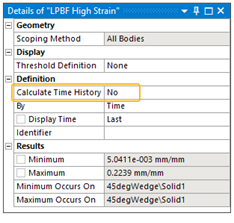
The LPBF High Strain result shows the maximum equivalent strain experienced during the build process. It can help to identify regions at risk of cracking.
Just as you do for the recoater interference result, consider defining a threshold for the level of strain that is considered to be of concern for your material. In the LPBF High Strain Details view, set the Threshold Definition to one of these options:
None (default) - The result tool will show pure maximum equivalent strain in the build, where the value at each point corresponds to the strain when that material was a new layer.
User Defined - You define your own warning and critical thresholds.
Once you have chosen your Threshold Definition, right-click the LPBF High Strain object and select Evaluate All Results. The resulting display shows the model with maximum equivalent strain values but with color contours based on the threshold criteria you selected. For the User Defined option, contours are shown as follows:
Blue = Safe
Green = Warning
Red = Critical
Note: To ensure a quick, dynamic calculation of results, Calculate Time History is set to No by default for this result item. Set Calculate Time History to Yes and then right-click Evaluate All Results to see the time history results, such as the layer-by-layer animated build. For large models, the calculation may take some time.
Check for Hotspots (Thermal-Structural System)
The LPBF Hotspot result is applicable for the thermal portion of an LPBF Thermal-Structural simulation. Use the result item after the thermal portion, at least, is solved.
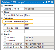
Right-click the LPBF Hotspot object and select Evaluate All Results. The resulting display shows the temperature of each layer right before the next layer is added. The worst hotspots are going to be the areas with the highest temperature for that layer.
Read-only result data show the minimum and maximum temperature values and where they occur (part or support).
Results are localized (based on nodal values), not averaged across the layer. Use a section plane to reveal hotspots inside the part.
Important: The data displayed is based on the temperature that the build cools down to at the end of each layer right before the next layer is added. It does not represent the "final state" of temperatures at the end of the cooldown step.
Note: To ensure a quick, dynamic calculation of results, Calculate Time History is set to No by default for this result item. Set Calculate Time History to Yes and then right-click Evaluate All Results to see the time history results, such as the layer-by-layer animated build. For large models, the calculation may take some time.
Scope a Line of Nodes to Get Results at a Specific Location
Suppose you want to obtain X-direction deformation along a line on a face of your part, such as shown below, at the end of the cooldown step.
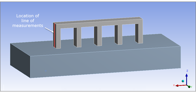
There are several ways to perform this function but we will demonstrate it using a Worksheet. To obtain distortion results along a line on the surface of your part:
Create a named selection: Highlight the Model object, right-click and select Insert > Named Selection. Right-click the newly created Selection object (under Named Selections) and Rename to something meaningful, for example, Line of Nodes.
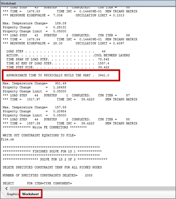
Get an Estimate of the Actual 3D Printing Time
View the solver output to get an estimate of the real machine build time. It is approximately the transient thermal build step simulation time multiplied by R^(1/3), where R is the number of deposit layers in one element layer. This data is available after the thermal solution. Click the Solution Information object and then click the Worksheet tab under the Geometry window. In the Details view, be sure that Solver Output is selected as Solution Output.