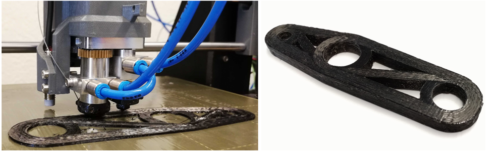
The following example has been provided by 9T Labs (https://www.9tlabs.com/) who automates and digitizes composite manufacturing. It shows how a 3D printed composite structure, designed with Fibrify, can be imported into Ansys Workbench/ACP for simulation. This workflow allows you to import a 3D composite lay-up definition and convert it into a solid FE model with minimal effort.

You can download the Workbench project archive here. You will find the required HDF5 Composite CAE file in the following location:

The model is already fully configured, and the description below highlights the most important steps.

Figure 4.56: 3D Printing with Endless Fiber Reinforcement and Final Part (Courtesy of 9T Labs)

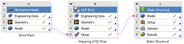
The following figure shows the Workbench Project Schematic. The 3D geometry of the printed composite part (shown above) is loaded into system A (Solid Mesh) and meshed in SpaceClaim. Three Named Selections are defined in Model A4 which are used to define the forces and supports later in the analysis system C3. This is important if you want to have an associative model. The material properties (such as stiffness and strengths) are defined in the Engineering Data component (B2) of the ACP Pre system. The solid mesh is transferred to ACP Pre by linking Model A4 with ACP Setup B5 which results in an Imported Solid Model in ACP Pre.

Figure 4.57: Simulation of a 3D Printed Composite (Courtesy of 9T Labs)

At this point, only a few mouse-clicks are needed in ACP Pre to load the 3D plies and to configure the mapping. You can perform the import using the context menu of the ACP Model as shown above (Figure 4.55: HDF5 Composite CAE Imported as 3D Plies (Imported Modeling Plies)). The imported plies are accessible in the object Tree and are displayed when selected. To see the Fiber Directions and other properties, enable the options in the display’s toolbar. Of course, the input data can be modified as well if needed.

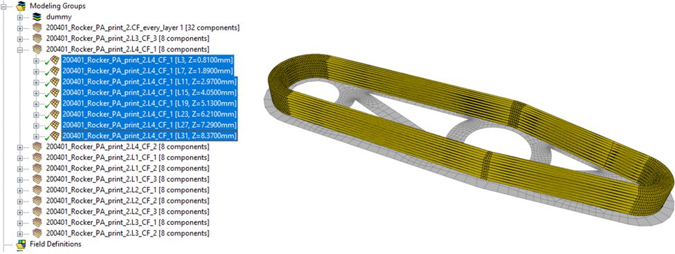
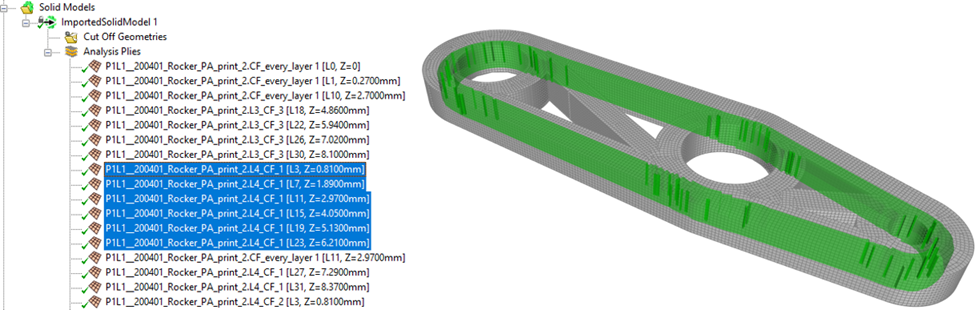
The solid mesh on which the plies are mapped is already available (mesh transfer from A4-B5). The mapping algorithm must be switched over to Imported Plies (3D plies) by enabling the Use Imported Plies option in the Imported Solid Model Property Dialog. By default, all plies are mapped and the result can be verified by selecting the plies of the solid model. The figure below shows a few plies which are visualized on the solid mesh. (Enable the Show on Solid option   in the display toolbar and select the plies.)

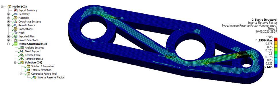
You can now transfer the solid mesh downstream for many different types of analyses, such as a static structural analysis as shown in System C in the workflow above ( Figure 4.57: Simulation of a 3D Printed Composite (Courtesy of 9T Labs)). After solving the analysis, you can employ the Composite Failure Tool to predict the safety margin of the composite part. As an example, the figure below shows the maximum Inverse Reserve Factor per element. Of course, you can easily generate ply-wise plots for a more detailed assessment.

Figure 4.58: Distribution of the Inverse Reserve Factors in the Mapped Composite Solid Model