


In earlier tutorials, you only used ACP (Post) for post-processing. Here, you will explore more options with Mechanical and other post-processing features in ACP (Post).
This section guides you through the following in Mechanical:
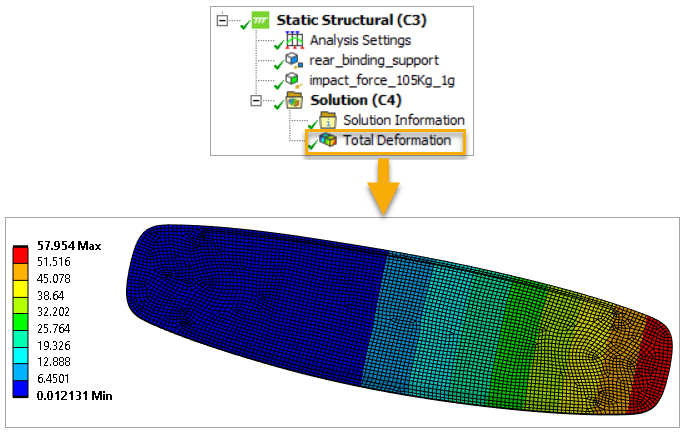
Adding a Total Deformation object in Mechanical provides a plot that corresponds to ACP (Post)'s deformation plot. Follow these steps to create a deformation plot using this object:
In the tree Outline, right-click Solution and select Insert. Select Deformation, then click Total.

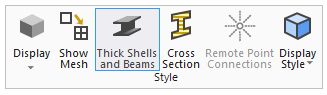
Switch to the Display tab, then select Thick Shells and Beams in the Style group.
Right-click Total Deformation object and select Retrieve This Result to visualize the plot.
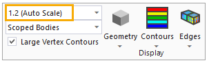
Note: The default deformation scale is 1.2 (Auto Scale). You can view and change this by navigating to the Display group of the Result tab.
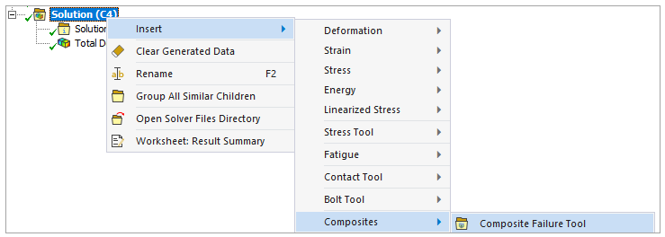
The Composite Failure Tool provides result data that corresponds to the failure definition in ACP (Post). Follow these steps to create a failure plot using this tool:
In the tree Outline, right-click Solution and insert a Composite Failure Tool under Composites.
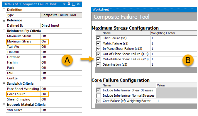
In the Details pane, switch Maximum Stress and Core Failure to On (A). In the Worksheet pane, configure the Maximum Stress and Core Failure properties as shown in the image below (B).
Expand Composite Failure Tool under Solution to check the Inverse Reserve Factor.
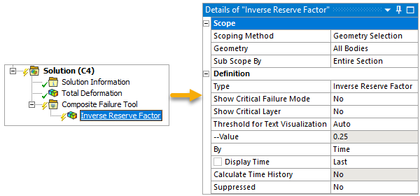
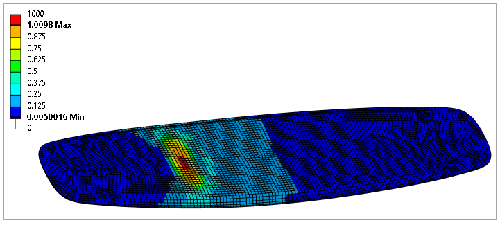
Right-click Inverse Reserve Factor and select Retrieve This Result to view the Composite Failure plot.
Note: You can use probes to identify result quantities at any point or locate the minimum/maximum value on an object. To do the former, select the result plot of interest, then go to the Result tab, click the Probe icon, and hover over the plot to obtain the result values. You can also click the object to create a probe annotation for the location of interest. To do the latter, go to the Result tab, click the Maximum and/or Minimum icon in the toolbar, and then select the result plot of interest.
Close Mechanical and go back to Workbench.
In the Basic Sandwich Panel Tutorial, you learned the basics of the deformation, stress, failure, and through-the-thickness plots. Here, you will review the concepts and use other features to analyze the results from those plots.
In this section, you will setup up ACP (Post), check the imported result file, then create a deformation plot.
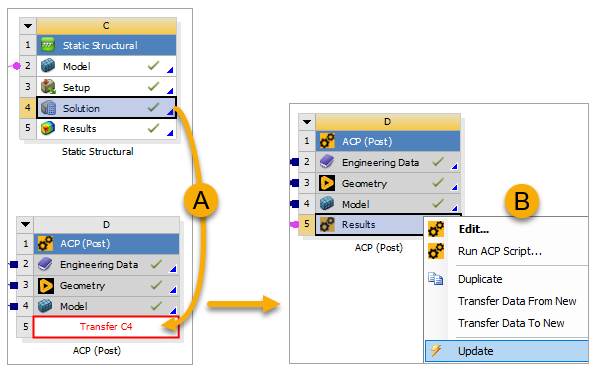
Under Component Systems in the Toolbox, click ACP (Post) and drop it onto the ACP (Pre) system.
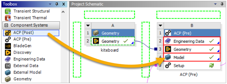
Click the C4 Solution cell and drop it onto the D5 Result cell to connect the two cells (A, below). Right-click the D5 Result cell and select Update (B), then double-click the cell to open ACP (Post).
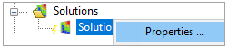
In the Tree View, expand Solutions, then right-click Solution 1 and select Properties.
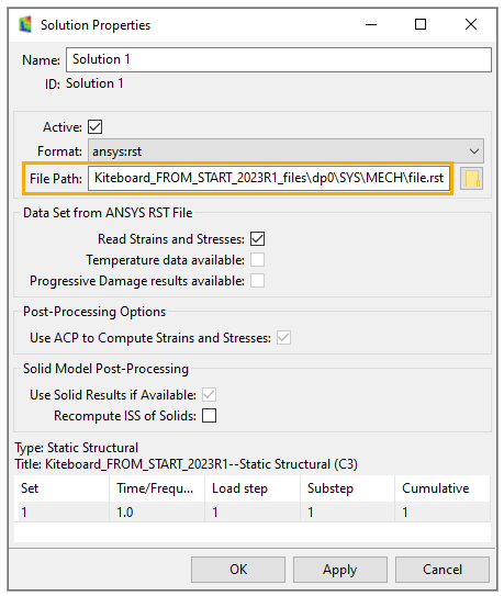
In the Solution Properties dialog, place the cursor in the File Path field to check that the result file was automatically inserted for post-processing. Close the dialog.
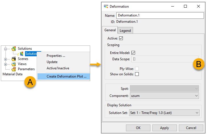
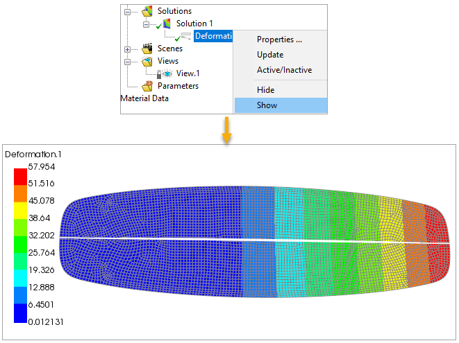
Right-click Solution 1 and select Create Deformation Plot (A, below). In the Deformation dialog, specify the properties as shown (B), then click Apply and close the dialog.
Under Solution 1, right-click Deformation.1 and select Show to visualize the plot on the model. Compare the result with that of the earlier section, Total Deformation in Mechanical.
ACP enables you to create stress plots for the composite model and individual Analysis Plies. You can also view the stress value of each element in the model and view different plot results when you change the stress type and component.
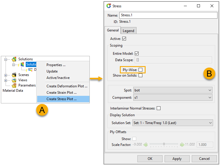
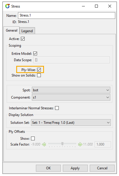
In the Tree View, right-click Solution 1 and select Create Stress Plot (A, below). In the Stress dialog, disable Ply-Wise then specify the properties as shown in the image (B). Click Apply and close the dialog.
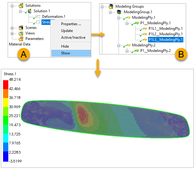
Under Solution 1, right-click Stress.1 and select Show to visualize the plot on the model. The plot shows the stress across all plies of the kiteboard.
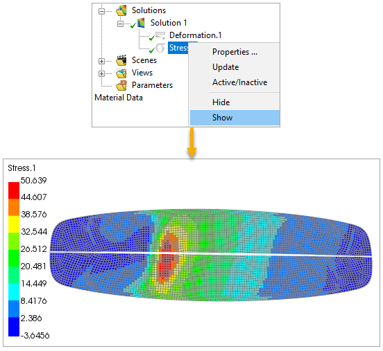
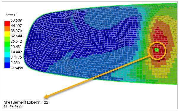
Select any element on the model to view the exact stress value of that element.
Double-click Stress.1 in the Tree View to open the Stress dialog. Enable Ply-Wise to view the stress result for each Analysis Ply.
Right-click Stress.1 and select Show (A, below). Expand Modeling Groups and click any Analysis Ply (B) to view the stress on that ply.
Tip: You can change the stress type and component by modifying Spot and Component in step 1 or 4 to see different stress results.
In this section, you will create a failure plot with the same failure criteria as the ones used in the earlier section, Composite Failure Tool in Mechanical. Similar to stress plots, failure plots enable you to examine the failure result of the whole structure, separate layers, or individual elements. You can also examine the failure modes, check on which plies the critical failures occur, and modify the plot legend.
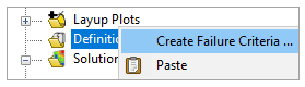
In the Tree View, right-click Definition and select Create Failure Criteria.
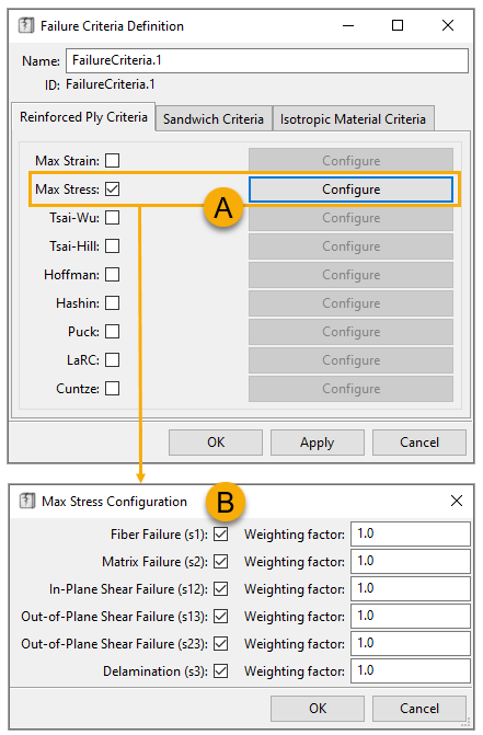
In the Failure Criteria Definition dialog, enable Max Stress, then click Configure (A). Specify the Max Stress properties as shown (B), then close the Max Stress Configuration dialog.
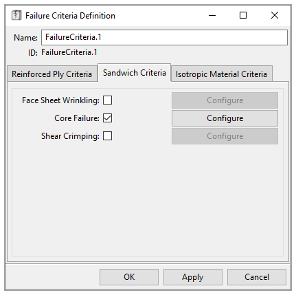
Switch to the Sandwich Criteria tab and enable Core Failure. Click Apply, then close the dialog.
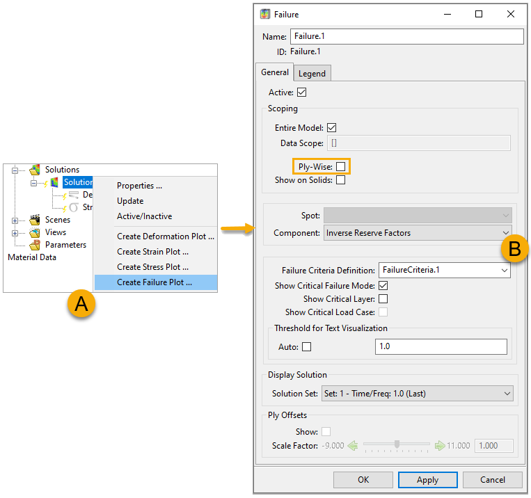
In the Tree View, right-click Solution 1 and select Create Failure Plot (A, below). In the Failure dialog, disable Ply-Wise then specify the properties as shown (B). Click Apply and close the dialog.
Tip: You can enable to view the failure results layer by layer.
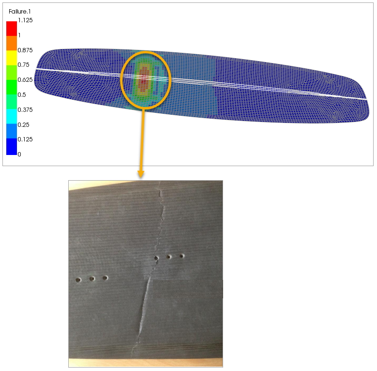
Right-click Failure.1 in the Tree View and select Show to visualize the failure result. The plot shows the failure across all plies of the kiteboard. The failure area corresponds with the failure in a real-life jump load testing scenario.
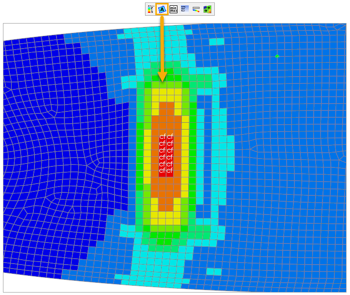
Activate the Toggle Text Plot icon on the toolbar to show the failure modes in the model.
Note: Failure Mode Notations
Maximum Strain e1t, e1c, e2t, e2c, e12 Maximum Stress s1t, s1c, s2t, s2c, s3t, s3c, s12, s23, s13 Tsai-Wu 2D and 3D tw Tsai-Hill 2D and 3D th Hashin
hf (fiber failure)
hm (matrix failure)
hd (delamination failure)
Puck (simplified, 2D and 3D)
pf (fiber failure)
pmA (matrix tension failure)
pmB (matrix compression failure)
pmC (matrix shear failure)
pd (delamination)
LaRC (2D)
lf (fiber failure)
lmt (matrix failure tension)
lmc (matrix failure compression)
Cuntze 2D and 3D
cft (fiber tension failure)
cfc (fiber compression failure)
cmA (matrix tension failure)
cmB (matrix compression failure)
cmC (matrix wedge shape failure)
Sandwich Failure Wrinkling
wb (wrinkling bottom face)
wt (wrinkling top face)
Sandwich Failure Core cf (core failure) Hoffman ho e = strain
s = stress
1 = material 1 direction
2 = material 2 direction
3 = out-of-plane normal direction
12 = in-plane shear
13 and 23 = out-of-plane shear terms
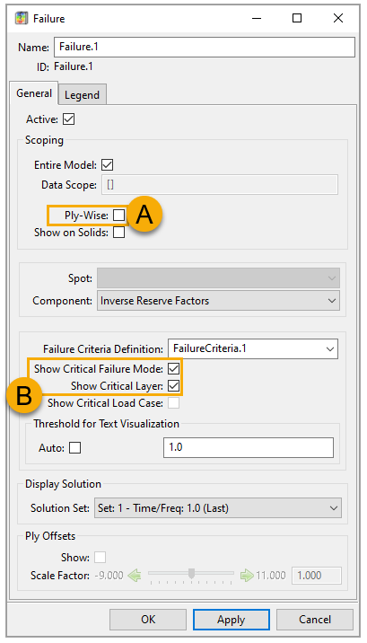
Double-click Failure.1 in the Tree View to open the Failure dialog. Ensure than Ply-Wise is unchecked (A, below). Enable Show Critical Failure Mode and Show Critical Layer (B). Click Apply, then close the dialog.
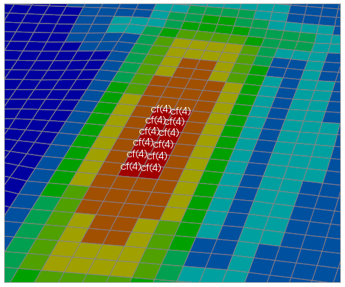
Zoom into the failure area of the model. The plot still shows the failure across all plies, but the annotation indicates that the core failures occur on ply 4.
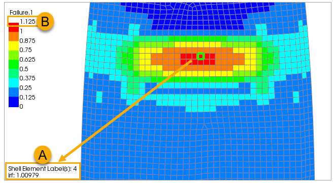
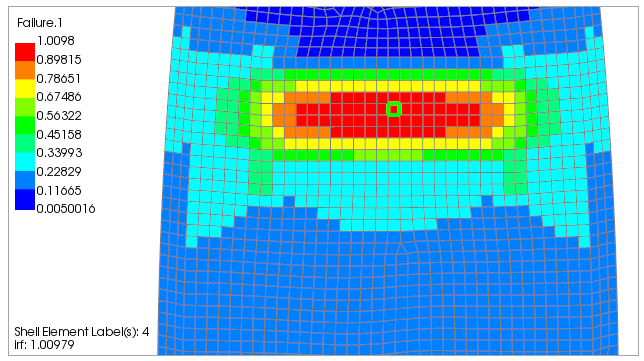
Select any element to view the exact failure value of that element. The maximum inverse reserve factor (Irf) value of this model is 1.00979 (A, below). However, the legend shows a maximum of 1.125 (B).
Open the Failure dialog and switch to the Legend tab. Uncheck Use Defaults (A, below) and try modifying the other properties to get different contour settings shown on the legend.
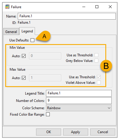
The setting shown in the image (B, above) results in more accurate maximum and minimum values on the legend. Compare the result with that of the earlier section, Composite Failure Tool in Mechanical.
To create a through-the-thickness plot to analyze a particular sampling point, follow these steps:
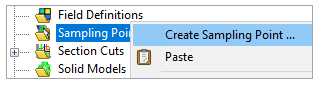
In the Tree View, right-click Sampling Points and select Create Sampling Point.
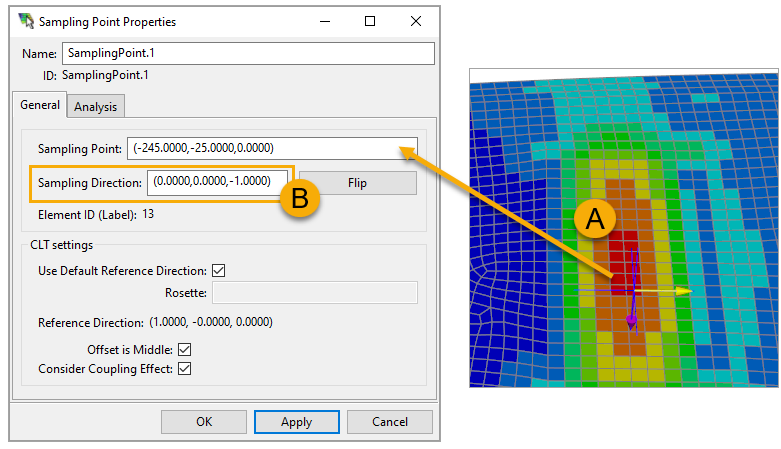
In the Sampling Point Properties dialog, place the cursor in the Sampling Point field, then select any element you want to analyze in the model (A). Specify the Sampling Direction as shown (B).
Switch to the Analysis tab. Specify the properties as shown in the image below. Click Stresses, then choose the stress type when the Edit properties dialog opens, and close the dialog. Click Apply to generate the plot.
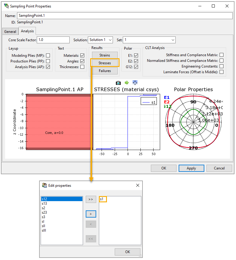
Change the stress type in step 3 to view a different stress plot or change the Sampling Point in step 2 to analyze a different element.