This section guides you through the following steps:
The project files are contained in a compressed file and can be downloaded here.
Once the download is complete, extract the compressed file. The folder contains two project archives: a from-start file and a solved file.
Start Ansys Workbench and Open the archive:
Basic_Sandwich_Panel_FROM_START_<release>.wbpz
Save the Workbench project.
Note: To check the result in the solved archive file:
Start Ansys Workbench and Open the solved archive: Basic_Sandwich_Panel_SOLVED_<Release>.wbpz.
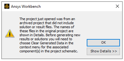
Close the warning dialog if it pops up.
Right-click the Model cell in the ACP (Pre) system, select Clear Generated Data, then click OK when the warning dialog pops up.
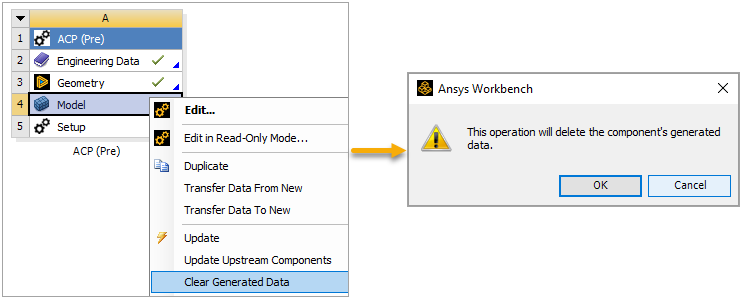
Click Update Project on the project toolbar.
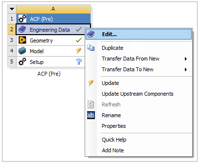
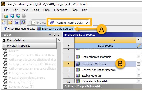
Right-click Engineering Data and select Edit from the menu.
As shown below, select Engineering Data Sources (A). Select Composite Materials (B) from the Data Source list.
You must now define the composite in Engineering Data. There are two ways to do this: you can import preconfigured materials from the Composite Materials catalog, or you can create new materials. In this example, you will do the latter, creating new materials as explained below.
Click Engineering Data Sources (C) to unhighlight that section. Then, under Contents of Engineering Data, manually add the name of the new material,
UD_T700(D).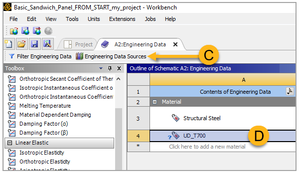
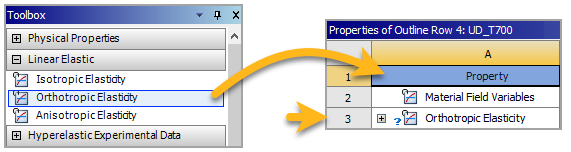
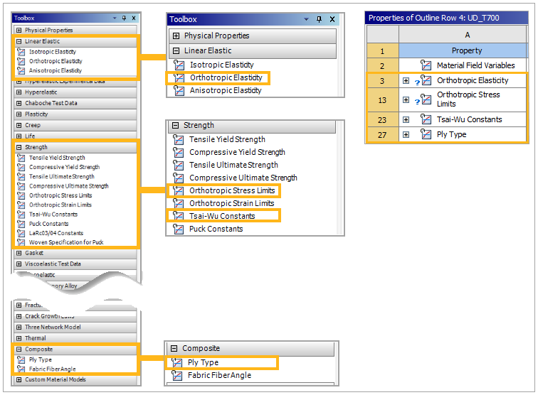
You will now create a new unidirectional (regular) material by dragging the required properties from the Toolbox onto the Properties cell as shown in the image below.
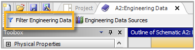
Tip: To display all properties, be sure to deactivate the Filter Engineering Data button above the Toolbox.
Add the following properties from the Toolbox:
Under Linear Elastic, add Orthotropic Elasticity.
Under Strength, add Orthotropic Stress Limits and Tsai-Wu Constants.
Under Composite, add Ply Type.
Assign a value to each material property as shown (A, below). The table below lists all the values to be entered.

Property (UD_T700) Value Unit Orthotropic Elasticity Young's Modulus X direction Young's Modulus Y direction Young's Modulus Z direction 1.15E+05
6430
6430
MPa
MPa
MPa
Poisson's Ratio XY Poisson's Ratio YZ Poisson's Ratio XZ 0.28
0.34
0.28
Shear Modulus XY Shear Modulus YZ Shear Modulus XZ 6000
6000
6000
MPa
MPa
MPa
Orthotropic Stress Limits Tensile X direction Tensile Y direction Tensile Z direction 1500
30
30
MPa
MPa
MPa
Compressive X direction Compressive Y direction Compressive Z direction -700
-100
-100
MPa
MPa
MPa
Shear XY Shear YZ Shear XZ 60
30
60
MPa
MPa
MPa
Tsai-Wu Constants Coupling Coefficient XY Coupling Coefficient YZ Coupling Coefficient XZ -1
-1
-1
Ply Type Type Regular Add the core material
Coracell_A550manually.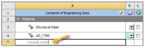
Add the following material properties from the Toolbox.
From Linear Elastic, select Isotropic Elasticity.
From Strength, select Orthotropic Stress Limits.
From Composite, select Ply Type.
Note:
Coracell_A550is a foam core. In most cases, foam materials have isotropic mechanical properties.Now assign a value to each material property according to the table below.
Property (Coracell_A550) Value Unit Isotropic Elasticity Derive from Young's Modulus and Poisson's Ratio Young's Modulus Poisson's Ratio Bulk Modulus Shear Modulus 85
0.3
70.833
32.692
MPa
MPa
MPa
Orthotropic Stress Limits Tensile X direction Tensile Y direction Tensile Z direction 1.6
1.6
1.6
MPa
MPa
MPa
Compressive X direction Compressive Y direction Compressive Z direction -1.1
-1.1-1.1
MPa
MPa
MPa
Shear XY Shear YZ Shear XZ 1.1
1.1
1.1
MPa
MPa
MPa
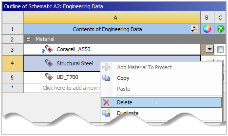
Ply Type Type Isotropic Homogeneous Core Since structural steel is not needed in this project, you may delete it from the Material list. Right-click Structural Steel and select Delete from the context menu.
To update the model, you must assign an arbitrary material and thickness to its geometry in Ansys Mechanical. Both properties will be overwritten in ACP later in the tutorial.
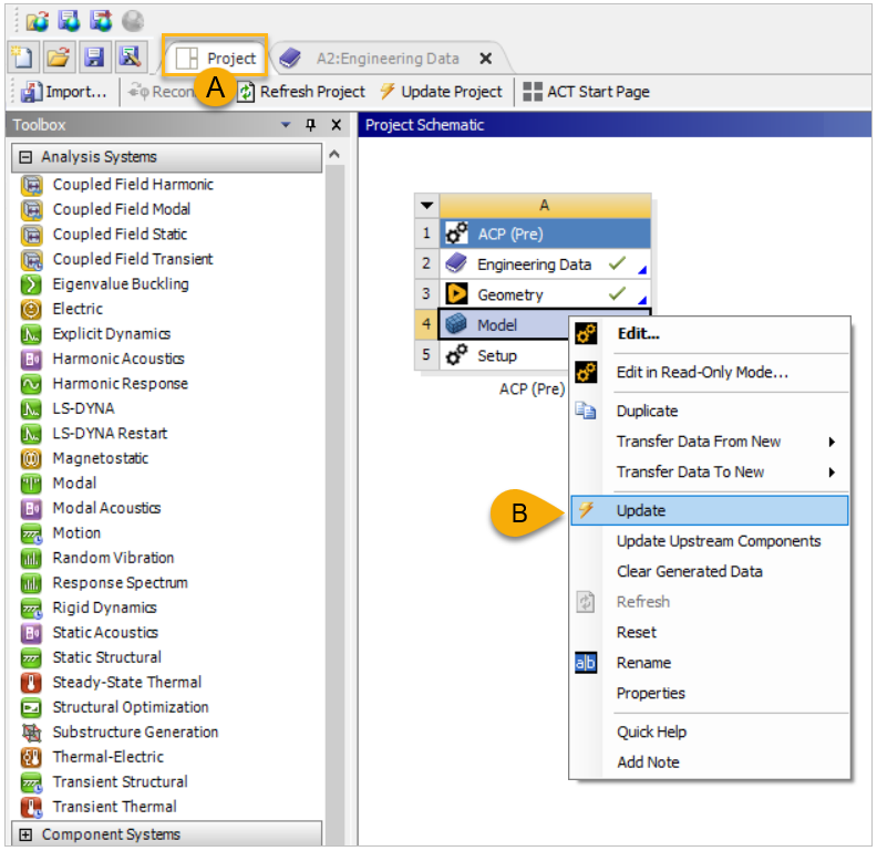
Return to the Project tab in Workbench and update the entire project.
Right-click the Model cell in ACP (Pre) and select Edit. In the opened window:
Expand Geometry in the Tree Outline. Select SYS-1/Sandwich Panel and assign a material and thickness to its Geometry.
Select the Mesh Face Sizing to assign its Geometry (then Type will automatically update).
Return to Ansys Workbench, right-click the Model cell, and select Update in the context menu.
You will now use ACP to further define the sandwich panel as explained in the following sections:
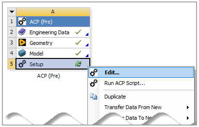
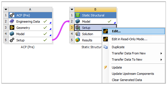
To open ACP, right-click Setup and select Edit from the context menu.
When ACP has launched, continue to define the material data:
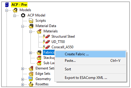
In ACP's Tree View, under Material Data, right-click Fabrics and select Create Fabric.
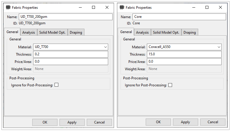
Create two new fabrics with the defined materials shown below. After you create the first fabric, click OK. Then repeat step 1 above to create the second fabric. Click OK.
Tip: The Weight/Area field will update to None as shown after you click OK.
Tip: Reorder the Tree View in ACP using keyboard shortcuts and mouse actions. Move items by:
Using the Copy (Ctrl+C) and Paste (Ctrl+V) keyboard shortcuts
Dragging one item onto another
A stackup is a multiaxial reinforcement tape consisting of several plies placed at different orientations. Typically, these layers are then stitch-bonded to form a fabric, also called a non-crimp fabric (NCF). See Creating Plies, to learn how fabric selection affects ply resolution.
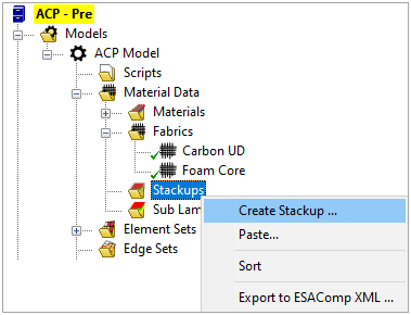
Right-click Stackups and select Create Stackup.
Define a new -45/+45 Stackup with the UD Biax Carbon.
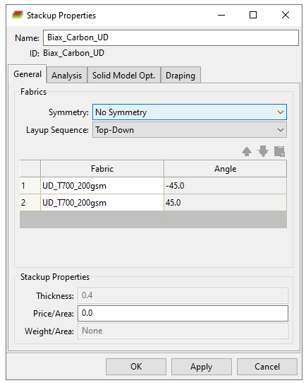
Click Apply. The calculated fields, Thickness and Weight/Area, will automatically update to the values shown above.
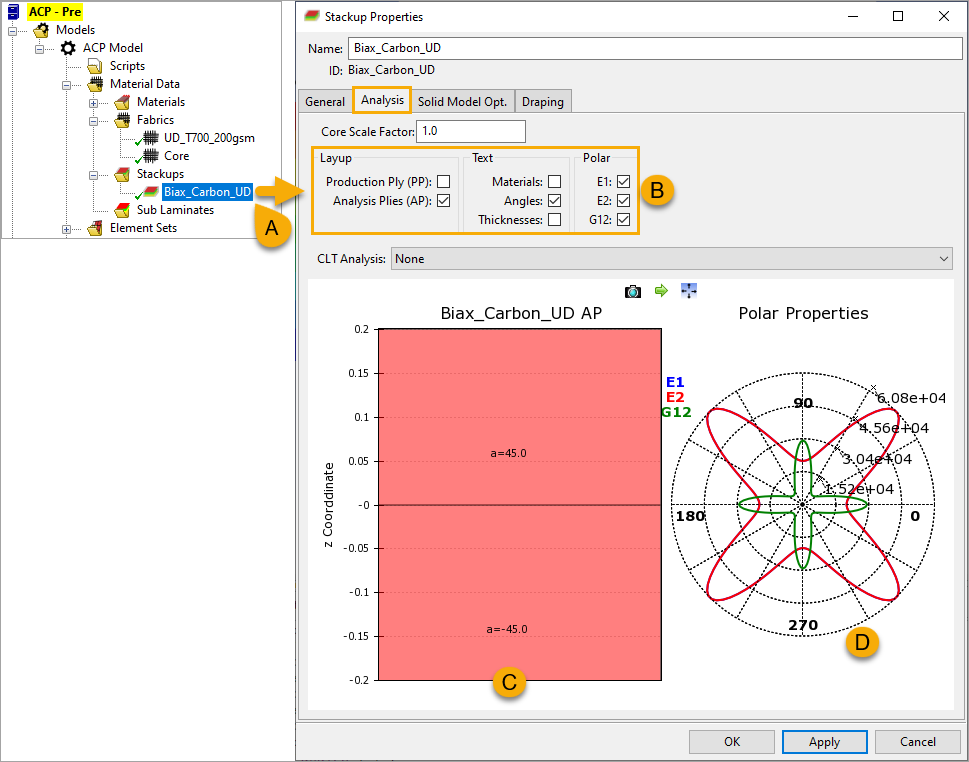
Click the Analysis tab in the Stackup Properties dialog where you created the
Biax_Carbon_UDstackup. Select the following analysis options as shown below (B):Under Layup, select Analysis Plies (AP).
Under Text, select Angles.
Under Polar, select E1, E2, and G12.
Click Apply to generate stackup information (C) and a polar properties plot (D).
Click OK to close the Stackup Properties dialog.
Sub Laminates group fabrics and stackups together. This speeds up modeling for recurring laminates.
Right-click Sub Laminates and select Create Sub Laminate from the context menu.
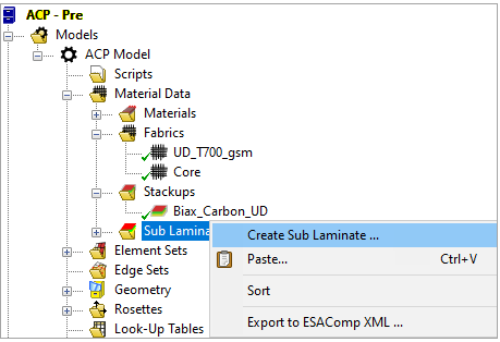
Combine the UD Biax Carbon stackup and UD T700 fabric into one Sub Laminate as shown below. Click Apply.
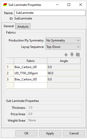
Click the Analysis tab. Again, generate stackup information and a polar properties plot as you did earlier (see Examining Stackup Properties). Select the Layup, Text, and Polar options shown below and click Apply.
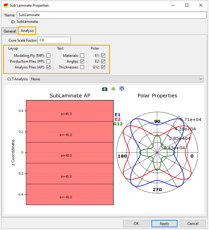
Click OK to close the dialog.
 A
rosette is a coordinate system that is used to set the reference direction (A
below) of an OSS, which specifies the direction (0°) all ply angles of an
MP are relative to. Both orientation and reference (B)
directions are important concepts in modeling composites.
A
rosette is a coordinate system that is used to set the reference direction (A
below) of an OSS, which specifies the direction (0°) all ply angles of an
MP are relative to. Both orientation and reference (B)
directions are important concepts in modeling composites.
To create a rosette:
In ACP, right-click Rosettes and select Create Rosette.
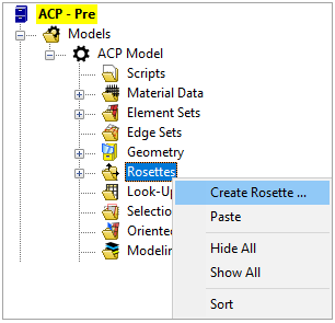
In the Rosette Properties dialog, specify the Origin (location of the rosette) and the 1 Direction and 2 Direction (the x and y directions of the rosette). There are two ways to do this: by manually entering the coordinates in their respective fields or by selecting a direction vector for the rosette. For the latter, hold Ctrl and select two element nodes. The direction vector aligns along the line between the two select element centers' respective nodes.
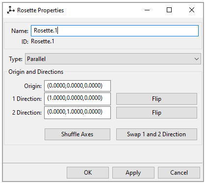
Click OK.
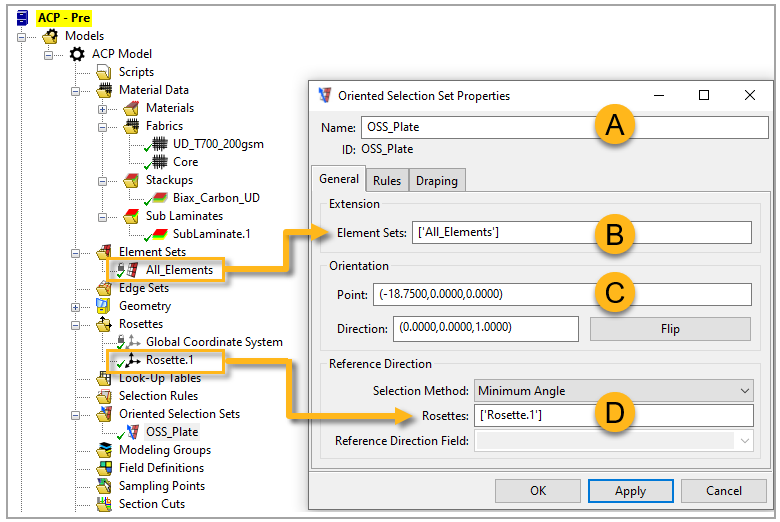
ACP uses the Oriented Selection Set (OSS) as part of the layup definition. The orientation direction of the OSS specifies the stacking direction of the modeling ply. The reference direction specifies the direction all ply angles are relative to.
The OSS concept creates independence from element properties such as element normal and element coordinate systems since plies are applied to the OSS and not on Element Sets. Mesh and element independence make ACP a powerful and flexible tool.
Right-click Oriented Selection Sets in the Tree View and select Create Oriented Selection Set.
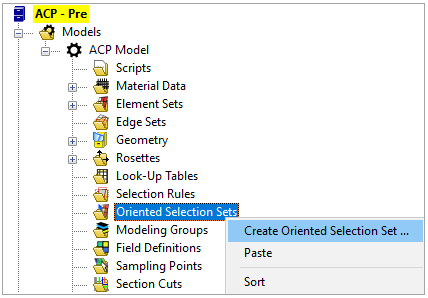
In the Oriented Selection Set Properties dialog, define the OSS as shown below:
Name: Enter
OSS_Plate.Element Sets: Place the cursor in the Element Sets field. Then click on All Elements (under Element Sets) in the Tree.
Point: Under Orientation, place your cursor in the Point field and then click an element or node that is within the mesh domain of the model.
Rosettes: Place your cursor in the Rosettes field. In the Tree, click the Rosette you made earlier to set the reference direction.
Click OK to close the dialog.
Tip:  Plot Properties is a useful feature in ACP. It adjusts
the scaling and amount of displayed vectors in the direction plots. This is
especially relevant when the mesh size is very fine. To view the various
other orientation visualization options, see Orientation Visualization in the ACP User's Guide.
Plot Properties is a useful feature in ACP. It adjusts
the scaling and amount of displayed vectors in the direction plots. This is
especially relevant when the mesh size is very fine. To view the various
other orientation visualization options, see Orientation Visualization in the ACP User's Guide.
A ply is a layer of material that is either a fabric, stackup, or sub laminate. The ply resolution indicates whether it is a modeling, production, or analysis ply.
A Modeling Ply (MP) is where the ACP lay-up is defined. The other two plies are built automatically from information placed on this level. For instance, a sub laminate is an MP and each of their materials (either fabric or stackup) displays as a PP.
A Production Ply (PP) derives from the Ply Material and Number of Layers in the MP properties. Fabric and stackup materials display as PP resolutions.
An Analysis Ply (AP) shows the plies used in the section definition for the Ansys solver. A PP without an AP indicates that the resulting AP contains no elements and is, therefore, not generated.
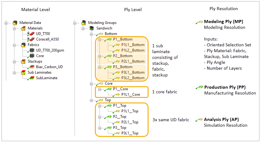
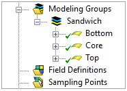
As shown in the Tree View below, the sandwich panel will have three plies: a bottom, core, and top. To create one, you must select an OSS, the ply material, the ply angle, and the number of layers. After each ply definition, you can update the ACP model to visualize the effect.
The following steps guide you through creating a Ply Group for the entire panel:
In the Tree, right-click Modeling Groups and select Create Modeling Group. In the Modeling Group Properties dialog, enter
Sandwichfor the Name. Click OK.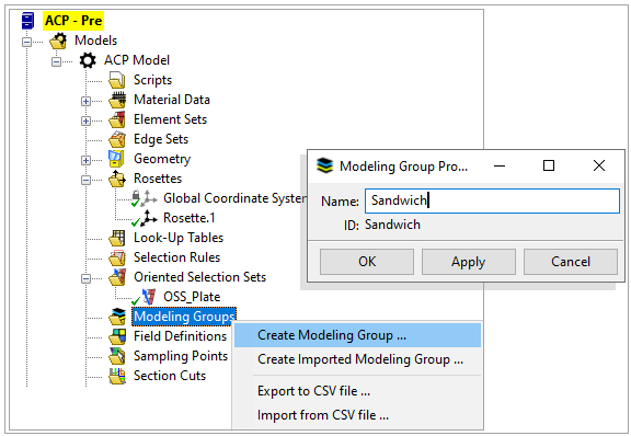
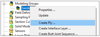
Right-click the new Sandwich group in the Tree and select Create Ply. This opens the Modeling Ply Properties dialog.
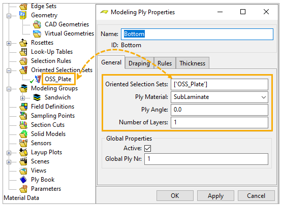
You will create three plies. Begin by creating the Bottom ply. In the Modeling Ply Properties dialog, enter the properties as shown in the image below. For the Oriented Selection Sets field, put the cursor in the field and click OSS_Plate in the Tree. When you have completed all the specified fields, click OK.
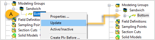
If you performed the previous steps correctly, the bottom ply will appear in the Tree under Modeling Groups/Sandwich. The lightning icon next to the Bottom ply (A, below) is a reminder to update the visual model so it reflects the changes. To do that, right-click Bottom and select Update from the context menu. The lightning icon will change to a green checkmark.
As you did in steps two through four, now create a Core ply and a Top ply. The table below lists the properties of each ply.
Ply Name Orientation Selection Sets Ply Material Ply Angle Number of Layers Notes 1 Bottom OSS_Plate Sublaminate 0.0 1 One sublaminate consisting of stackup, fabric, stackup. 2 Core OSS_Plate Core 0.0 1 One core fabric 3 Top OSS_Plate UD_T700_200gsm 90 3 Same UD Fabric, 3x 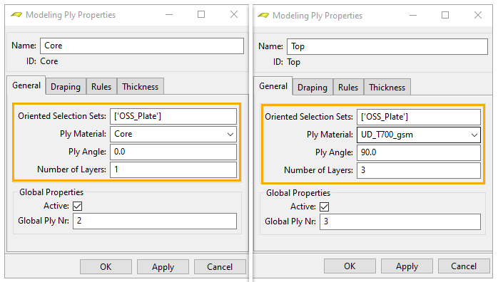
Tip: To rename an item in ACP's Tree View, you can click the item and then press F2.
This next section of the tutorial will guide you through the following steps in preparation for running an analysis in Ansys Mechanical.
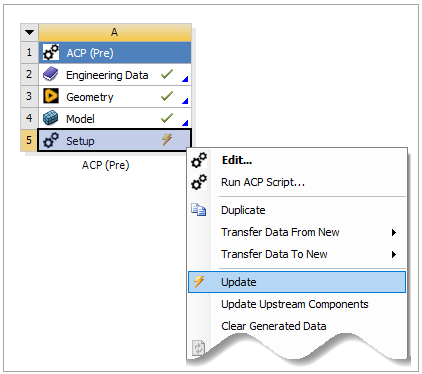
Return to the Workbench application. If there is a lightning icon in the Setup cell of the ACP (Pre) system, right-click the Setup and select Update in its context menu.
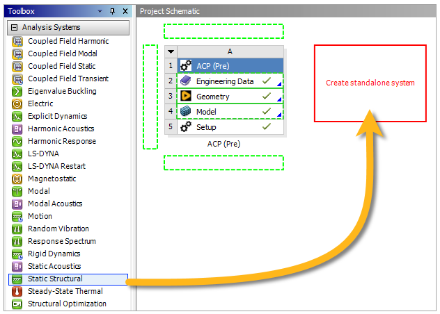
Now add a Static Structural system to the existing analysis.
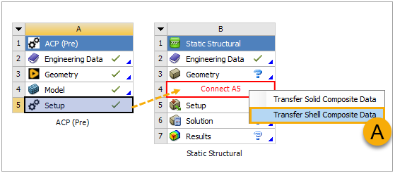
Connect the A5 Setup cell to the B4 Setup cell. (Click and drag from A5 to B4.) Choose the option Transfer Shell Composite Data (A, below).
Update the Model cell of the Static Structural system.
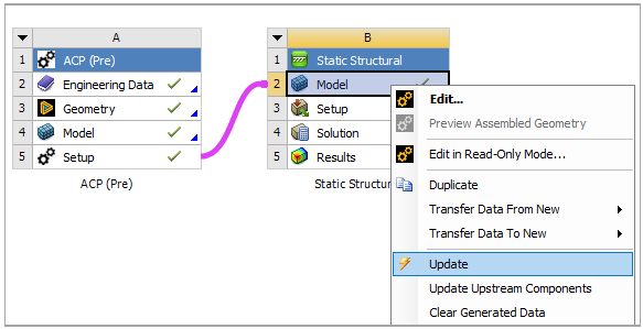
Right-click the B3 Setup cell and select Edit in the context menu. This will open Ansys Mechanical.
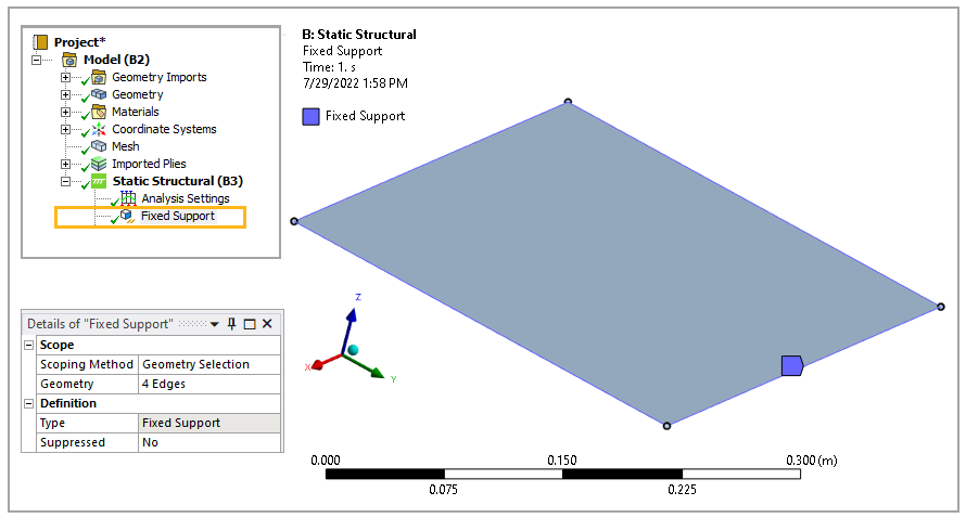
Insert a Fixed Support to the system. Then add it to the edges of the panel by choosing the select icon in the toolbar. Click the first edge and select the Apply Selection icon. Add the other three edges to the Geometry scope by clicking on them and selecting the Add To
 icon.
icon.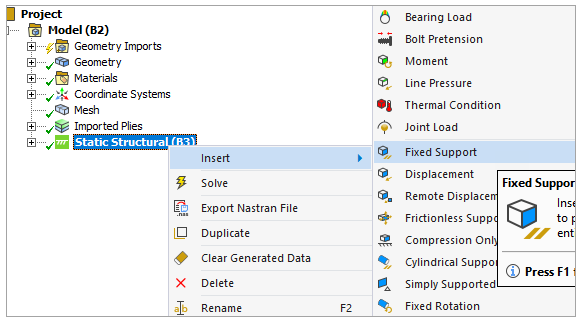
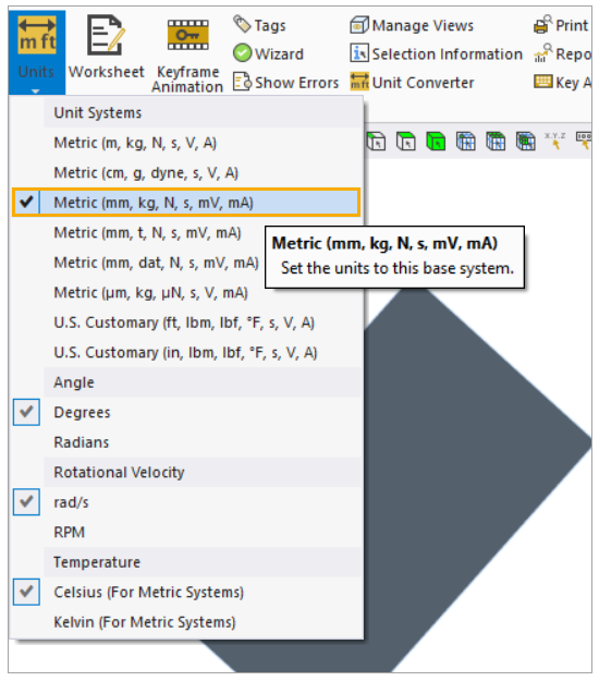
If needed, set the units to the millimeter base system by clicking the Units icon on the toolbar and selecting Metric (mm, kg, N, s, mV, mA).
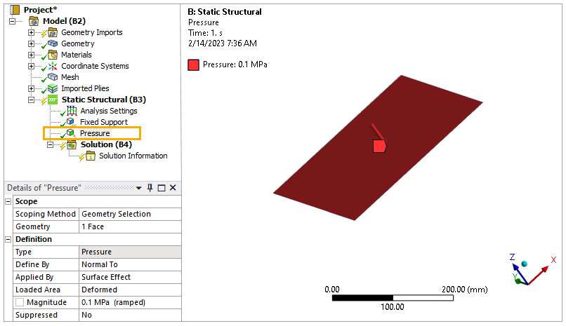
Add an applied load onto the panel and specify the properties as shown below.
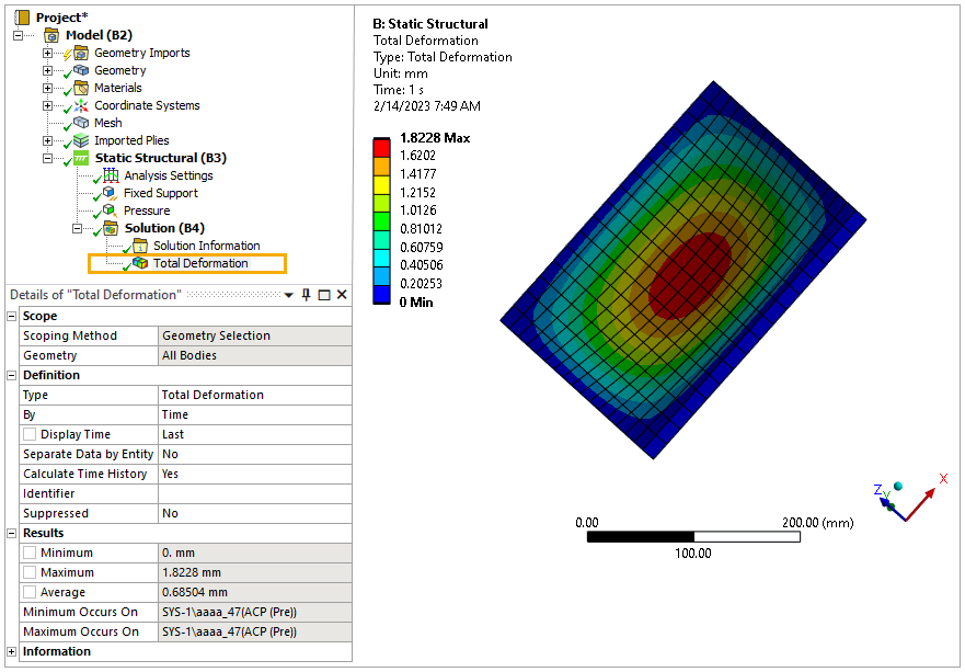
Solve the analysis in Ansys Mechanical by right-clicking Solution and selecting Solve.
Following the analysis, create the total deformation plot of the sandwich panel. To visualize it, right-click Total Deformation and select Retrieve This Result.