Creating a 3D Energy Density Sensor
This page shows how to create a 3D Energy Density Sensor. This sensor allows you to compute the absorbed energy density in Lumen/m3 or Watt/m3 which can be useful when working with highly diffusive materials, wanting to track some hot spots or wanting to visualize the rays' distribution inside the volume itself.
Important: This feature is only available under Speos Premium or
Enterprise license.
To create a 3D Energy Density Sensor:
-
From the Light Simulation tab, click 3D Energy
Density
_Sensor_3D_Energy_Density.png) .
The sensor appears in the 3D view and is placed on the origin of the assembly.
.
The sensor appears in the 3D view and is placed on the origin of the assembly. -
If you want to modify the axis system of the sensor, click
_Origin_Point.png) to select the origin,
to select the origin, _Sensor_Axis_X.png) to define the X axis and
to define the X axis and _Sensor_Axis_Y.png) to define the Y axis or click
to define the Y axis or click _Axis_System_Autofill.png) and select a coordinate
system to autofill the Axis System.
Note: If you define manually one axis only, the other axis is automatically (and randomly) calculated by Speos in the 3D view. However, the other axis in the Definition panel may not correspond to the axis in the 3D view. Please refer to the axis in the 3D view.
and select a coordinate
system to autofill the Axis System.
Note: If you define manually one axis only, the other axis is automatically (and randomly) calculated by Speos in the 3D view. However, the other axis in the Definition panel may not correspond to the axis in the 3D view. Please refer to the axis in the 3D view. -
From the Layer drop-down list:
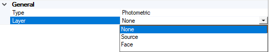
- Select None to get the simulation's results in one layer.
-
Select Source if you have created more than one source and want to include one layer per active source in the result.
Tip: You can change the source's power or spectrum with the Virtual Lighting Controller in Virtual 3D Photometric Lab. -
Select Face to include one layer per surface selected in the result.
Tip: Separating the result by face is useful when working on a reflector analysis.-
In the 3D view click
_Sensor_Contributing_Faces.png) and select the
contributing faces you want to include for layer separation.Tip: Select a group (Named Selection) to separate the result with one layer for all the faces contained in the group.
and select the
contributing faces you want to include for layer separation.Tip: Select a group (Named Selection) to separate the result with one layer for all the faces contained in the group. - Select the filtering mode to use to store the results (*.xm3):
_Sensor_Filtering_Mode.png)
- Last Impact: with this mode, the ray is integrated in the layer of the last hit surface before hitting the sensor.
- Intersected one time: with this mode, the ray is integrated in the layer of the last hit selected surface if the surface has been selected as a contributing face or the ray intersects it at least one time.
-
-
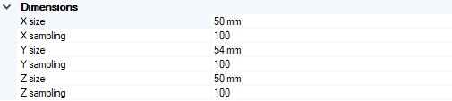
Adjust the sampling of the sensor on X, Y and Z axes.