
Adding a Solution Setup to an HFSS with Hybrid and Arrays Design
If you have an existing setup an HFSS with Hybrid and Arrays solution type, you can Copy and Paste it, and then edit parameters. If you have already created a solution and you want to use an existing mesh, you can click Add Dependent Solve Setup. To add a new solution setup to a design:
- Select a design in the project tree.
- Click HFSS>Analysis Setup>Add
Solution Setup, or right-click Analysis
in the project tree, and then click Add Solution
Setup on the shortcut menu, or select the Simulation tab on the ribbon, and click the Setup icon:
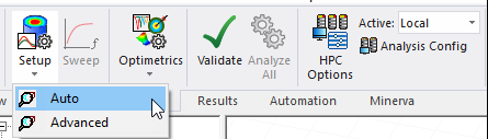
For HFSS with Hybrid and Arrays solutions, you can choose Auto or Advanced Solution Setup.
Auto Solution Setup
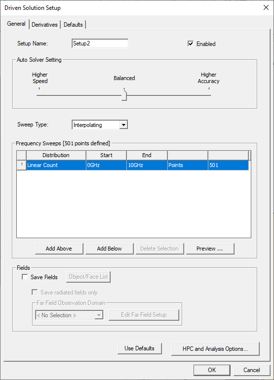
In order to use Auto setup, "Use Automatic Settings" under Analysis Configuration must be checked. Auto features a simplified dialog with a slider bar that you can adjust from Higher Speed (which sacrifices accuracy to achieve optimum speed), to Balanced (which is more accurate but faster than the highest accuracy setting) to Higher Accuracy (which takes the time to ensure optimal accuracy). These settings also apply to any FEBI or IE Regions that use the IE Solver in a design.
The Properties for the Auto Solver Setting includes the same choices.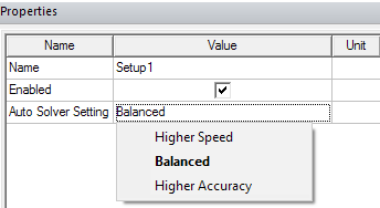
The Auto setup includes a single sweep, for which you can edit the Distribution, Start, and End. If the design does not include a port, the sweep type can only be Discrete. If one or port ports exist, the sweep can be Interpolating or Discrete.
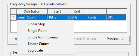
- You specify sweeps in terms of Distribution type, which can be Linear Step, Linear Count, Log Scale, Single Point , or Single Point Sweep, which adds a set of 10 Single Point Sweeps, defaulting from 1 GHz to 10 GHz in increments.. The Add Above, and Add Below buttons permit you to add additional sweeps, including mixed sweep types. This feature provides flexibility. For example, you can define sweeps with log scale at lower frequencies, and linear step at higher frequencies.
If you add more sweeps, you can Delete a selected distribution.
The Preview button displays the sweep(s) as currently defined.
The Auto setup includes tabs for General, Derivatives, and Defaults.
|
General |
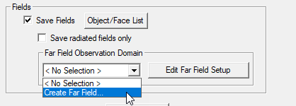
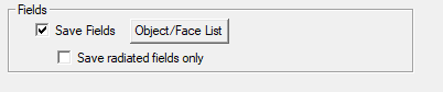
Includes general solution settings. You can specify the name, change the slider bar to do different solver settings, choose sweep type, set frequency range, choose Save Fields and Save radiated fields only options, (required if you intend to Plot Field Overlays) and do HPC settings. Includes settings for mesh linking, mesh assembly for designs that include 3D components, absorbing boundaries on ports, wave port adapt options, and whether to Save Fields and Save radiated fields only. You must save fields if you intend to plot or post process fields. For HFSS solutions without Hybrid Regions, the Fields area contains a Far Field Observation Domain area that allows you to specify a Far Field sphere or edit an existing setup. To evaluate radiated fields in the far-field region, you must check Saved Fields in the solution and sweep setups, and set up an infinite sphere that surrounds the radiating object. You can set up the infinite sphere by selecting Create Far Field... from the menu. For the procedure, see Setting up a Far Field Infinite Sphere.
If you do so, fields are generated during the solve and for any dependent frequency sweeps, and written as .ffd files rather than as a post processing step. After the simulation, editing or deleting the selected far field setup invalidates the last adaptive solution of the driven setup as well as its dependent sweep’s solution. If an HFSS with Hybrid and Arrays project contains an SBR+ Hybrid Region, the Fields area does not contain the Fields Observation Domain area.
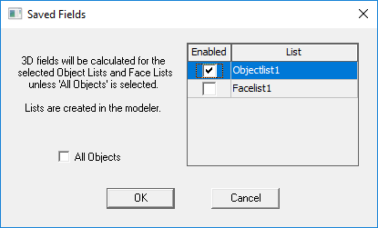
For very large designs, especially for finite array designs, saving fields can potentially result in very large files. In such cases, you can use the Object/Face List button to open a Saved Fields dialog to select from object or face lists you have predefined. You would then save 3D fields only on certain objects or faces, which could save disk space. The default is All Objects. The selection in the solve setup will dictate the behavior of the frequency sweep solve. Changing the selected lists will invalidate the last adaptive solution. If you subsequently create a Near Field or Far Field Radiation setup and select a list there, you receive a warning if your selections do not match those selected for the solve. For very large designs, especially for finite array designs, this can potentially result in very large files. In such cases, you can use the Object/Face List button to select from object or face lists you have predefined. You would then save 3D fields only on certain objects or faces, which could save disk space. The selection in the solve setup will dictate the behavior of the frequency sweep solve. Changing the selected lists will invalidate the last adaptive solution. If you subsequently create a Near Field or Far Field Radiation setup and select a list there, you receive a warning if your selections do not match those selected for the solve. |
|
Derivatives |
If your design contains variables, they are listed here. HFSS can calculate derivatives for your variables. |
|
Defaults |
Enables you to save the current settings as the defaults for future solution setups or revert the current settings to HFSS's standard settings. |
Advanced Solution Setup
The Advanced Solution Setup lets you have more control over the settings, and provides more options. For all HFSS solution types, if you choose Advanced, the Solution Setup
dialog box appears. The appearance differs depending on the Solution Type. For example for Driven Solution Terminal Types, the DC R (Beta) tab also appears.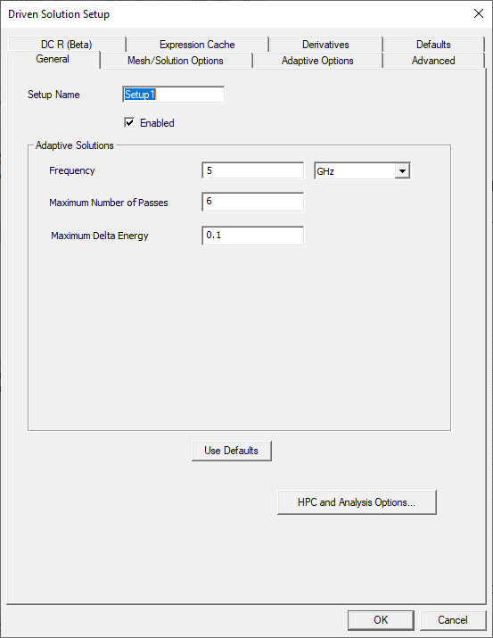
It is divided among the following tabs:
|
General |
Includes general solution settings, including frequency and S-parameter settings. |
|
Mesh/Solution Options |
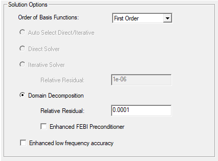
Includes settings for lambda refinement, adaptive analysis and solution options, the Order of Basis setting, whether to use the direct solver or iterative solver, whether to enable the use of solver domains, if available for the solution type, and for designs that contain only lumped ports as sources, or a combination of lumped and circuit ports, whether to use Enhanced low frequency accuracy. In those cases, when you enable Enhanced low frequency accuracy the solver is tuned to reliably solve low frequencies. In addition, for designs with only lumped ports and/or circuit ports, interpolating sweeps are tuned to solve more low frequency points in order to accurately represent very low frequency results. In the case of a design that includes a 3D Component Array and a FE-BI Hybrid Region, the Mesh/Solution options includes an option to select Enhanced FEBI Preconditioner.
When an HFSS 3D Component Array design has a FEBI region, the setup only allows you to select the Domain Decomposition solver. The Enhanced FEBI Preconditioner allows you to achieve faster simulation speed for most cases, at the cost of more memory. |
|
Advanced |
Includes settings for mesh linking, mesh assembly for designs that include 3D components, absorbing boundaries on ports, wave port adapt options, and whether to Save Fields and Save radiated fields only. You must save fields if you intend to plot or post process fields. For HFSS with Hybrid and Arrays solutions that do not contain SBR+ Hybrid Regions, the Fields area contains a Fields Observation Domain area that allows you to specify a Far Field sphere or edit an existing setup. If you do so, fields are generated during the solve,
If you do so, fields are generated during the solve and for any dependent frequency sweeps, and written as .ffd files rather than as a post processing step. After the simulation, editing or deleting the selected far field setup invalidates the last adaptive solution of the driven setup as well as its dependent sweep’s solution. If an HFSS project contains an SBR+ Hybrid Region, the Fields area does not contain the Fields Observation Domain area.
For very large designs, especially for finite array designs, saving fields can potentially result in very large files. In such cases, you can use the Object/Face List button to open a Saved Fields dialog box to select from object or face lists you have predefined. You would then save 3D fields only on certain objects or faces, which could save disk space. The default is All Objects. The selection in the solve setup will dictate the behavior of the frequency sweep solve. Changing the selected lists will invalidate the last adaptive solution. If you subsequently create a Near Field or Far Field Radiation setup and select a list there, you receive a warning if your selections do not match those selected for the solve. |
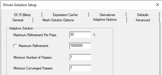
| Adaptive Options |
The Adaptive Options include Maximum Refinement per pass, Maximum Refinement, and Minimum Number of Passes, and Minimum Converged Passes.
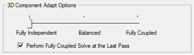
Minimum Number of Converged Passes If you have set the Beta Option for Parallel Component Mesh Adapt, and the design contains 3D components, the Adaptive Options tab also lets you select 3D Component Adapt Options.
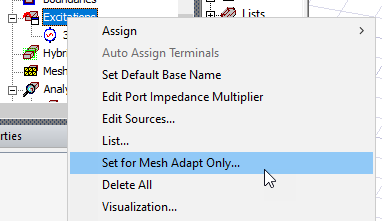
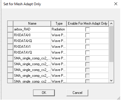
Parallel component adapt for mesh fusion workflow in MCAD including both 3D component array and general mesh fusion. During the component adapt, the multiple components are solved in parallel during each adaptive pass. You can select from Fully Independent adapt (the default for a Mesh Fusion project), Balanced adapt, and Fully coupled adapt. If you select Fully Independent or Balanced, you can specify that the last adaptive solve performs a Fully Coupled Solve, or if unchecked, a memory estimation. You can assign certain boundaries and ports to improve adaptive accuracy. For example, for component without any ports, certain ports together with a PEC boundary can be added to drive the adaptive pass. These boundaries and/or ports are present during adaptive pass only and will be removed automatically during full design solve. To do so, right-click on the Excitations icon and select Set for Mesh Adapt Only...
This opens a dialog listing the ports/boundaries.
When an adapted port is present, you have an option to display s-parameter results that do or do not include adapted ports (full s-matrix or reduce s-matrix) for adaptive solves. Ports selected here do not appear in the Edit Sources dialog. Because there is no LastAdaptive solution if you turn off “Perform Fully Coupled Solve at the Last Pass”, the far field plot will be blank. |
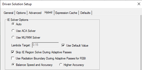
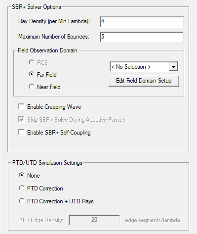
| Hybrid |
If the design includes Hybrid regions, this tab for Setting Hybrid Parameters for HFSS.
If SBR+ Regions are present, you can set SBR+ Solver Options.
|
|
Expression Cache |
Includes a list of expressions (including post processing variables) that you can use for convergence for adaptive analysis. |
|
Derivatives |
If your design contains variables, they are listed here. HFSS can calculate derivatives for your variables. |
|
Defaults |
Enables you to save the current settings as the defaults for future solution setups or revert the current settings to HFSS's standard settings. |
- Click the General tab.
- The Enabled check box on General tab permits to you to disable a setup so that it does not run when you select Analyze All.
- For Driven solution types, do the following:
- Select whether you want to solve for Single frequency, Multi-Frequency, or Broadband, and enter the appropriate Solution Frequency data and select the frequency units from the pull down list.
- Optionally, select Solve Ports Only.
- The lower right corner also contains a button for HPC and Analysis options. Here you can select or create an analysis configuration.
- Click OK.
- Optionally, add a frequency sweep to the solution setup.