Computing Near Fields

To analyze the radiated fields associated with a design, a radiation surface is defined over which the fields are calculated. The values of the fields over this surface are used to compute the fields in the space surrounding the device. This space is typically split into two regions: the near-field region and the far-field region. The near-field region exists at less than a wavelength from an energy source. The far-field region is where radiation occurs. Both near and far fields can play a role in EMI. Near and far field analyses can use sources defined in SIwave or via push excitations from Ansys Electronics Desktop.

To perform a near field simulation:

1. Click Simulation.
2. From the SIwave area, click Compute Near Field.

The Compute Near Field window appears.



3. From the Simulation name field, enter a name for the simulation.

4. From the Excitations area, select a source of excitations (i.e., Use sources defined in the project or Use sources defined in external file. If users select Use source defined in external file, Browse to an appropriate file and select it. Then, if appropriate, check the Interpolate spectrum at missing frequency points box.

5. From the Frequency Range Setup area, click the Start Freq., Stop Freq., and Num. Points fields to enter values.

6. Use the Distribution drop-down menu to select either Linear or By Decade.
   • Linear – the difference between the start frequency and the stop frequency is calculated and is divided by the number of solution points.
   • By Decade – distributes the number of points specified logarithmically, over each decade.

7. If appropriate, add or remove rows to the Frequency Range using the Add Above, Add Below, and Delete Selection buttons.
8. If appropriate, click Save to save the settings as a SIwave Frequency Sweep Distribution File (*.sfsdf). Click Load to choose previously saved settings. 
9. If appropriate, click Set Default to set the current grid settings as a default value for that simulation type. When a default value has been set, the window for that simulation type will always be populated with those settings when the window is opened. Click Clear Default to remove the default setting and return the population of the grid to its normal behavior.
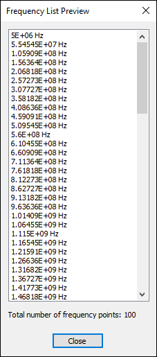
10. Click Preview... to open the Frequency List Preview window.



11. From the Meshing Frequencies for the Observation Mesh area, use the radio buttons to select which frequencies will be used for the observation mesh:
    • Default – uses the default max. frequency from the sweep (5Ghz).
    • Points – opens menu options that allow you to enter specific frequencies.
    • Range – opens menu options that allow you to select a start and stop frequency.
12. From the Cuboid Surface Positions area, enter values for +x, -x, +y, -y, +z, and -z offset. These values define a cuboid that completely encloses the design by specifying the cuboid face offset values from the design bounding box. The near field is evaluated on the surface of this cuboid.



Note:

Offsets that are very small may increase simulation time.

13. From the Near Field Solver Options area, enter values for the following:
    1. Min. Adapt Passes – an adaptive analysis will not stop unless the minimum number of passes specified is completed, even if convergence criteria have been met.
    2. Max. Adapt Passes- this value is the maximum number of mesh refinement cycles SIwave will perform. This value is a stopping criterion for the adaptive solution; if the maximum number of passes has been completed, the adaptive analysis stops; otherwise, the adaptive analysis will continue unless the convergence criteria are reached.
       Note:

       The size of the finite element mesh — and the amount of memory required to generate a solution — increases with each adaptive refinement of the mesh. Setting the maximum number of passes too high can result in SIwave requesting more memory than is available or taking excessive time to compute the solutions.

    3. Triangles to Add/Pass
    4. Global Error Tolerance – this is the maximum relative difference allowed between two successive passes.
14. From the Maximum Edge Length area, use the radio buttons to select Automatically determined or enter a value in mils. SIwave generates a surface triangular mesh such that the triangle edge lengths are equal to or less than the specified value.
15. If appropriate, check Export near field data to .and/.nfd files after simulation completes and select a location for the file. Near field data is exported in Ansys Nearfield Data (*.and) format, and can be used as external incident field data in Ansys HFSS simulations.
16. If appropriate, click Save settings to save these values.
17. If appropriate, click Other solver options to change general solver options.
18. Click Launch to begin simulation.

The Messages window opens a Process Monitor tab that displays the progress.