Eddy Current Solver Settings

The settings available in the Eddy Current Solve Setup\Solver tab are determined by the type of design selected (2D, 3D T-W, or 3D A-F).

For an Eddy Current 2D Solution:

1. Adaptive Frequency – This value specifies the nominal problem frequency, which will be used in the adaptive mesh process. The units are specified by the user. The value can be specified using variables and expressions.
2. Nonlinear Residual – This value specifies how close each solution must come to satisfying the equations that are used to compute the electric field.
3. Smooth BH Curve – This option allows the solver to smoothen the list of points to make a refined BH curve for better solving. If this option is not selected, the solver just uses the discrete points.
4. Number of Nonlinear Iterations – This provides an option for you to set both a Minimum iteration number to avoid non-converged solution, and a Maximum iteration number to avoid taking too much computation time. These values must be integers greater than 0. By default the values for Minimum and Maximum are 1 and 100, respectively. Maximum number should be greater than the Minimum number.
5. Thermal Two-Way Coupling\Relaxation – This setting can be used to improve two-way coupling convergence by applying the relaxation factor to the temperature field. When the thermal modifier takes on a nonlinear form, the convergence of the solution field in Maxwell's equations may fail during two-way coupling iterations. With nonlinear iterations, using an under-relaxation factor can mitigate the risk of overshooting in the property updating process.

The range of the relaxation factor is from 0 to 1. In general, a smaller relaxation value helps convergence, but may increase the total number of iterations. The default relaxation factor is 1.0.

The Thermal Two-Way Coupling\Relaxation setting is applicable only when Enable Feedback is checked in Temperature of Objects window, which invokes two-way coupling instead of one-way coupling. The relaxation setting is

• applicable to all Maxwell 2D designs,
• applicable to both geometry modes (Cartesian XY and Cylindrical about Z),
• does not support non-intrinsic and intrinsic variables.

If activated in the Solve Setup window, the Relaxation Factor is also available in the Solve Properties window: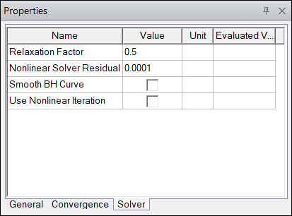


6. If desired, you can Import Mesh.

For an Eddy Current 3D T-W Solution:

1. Adaptive Frequency – This value specifies the nominal problem frequency, which will be used in the adaptive mesh process. The units are specified by the user. The value can be specified using variables and expressions.
2. Nonlinear Residual – This value specifies how close each solution must come to satisfying the equations that are used to compute the electric field.
3. Smooth BH Curve – This option allows the solver to smoothen the list of points to make a refined BH curve for better solving. If this option is not selected, the solver just uses the discrete points.
4. Enable an Iterative Solver – This option enables the iterative solver, rather than the direct solver. For more information, see Interative Matrix Solver.

5. Use higher order shape functions – This optional setting will increase the order of electric vector potential to 2 from the default order of 1. Enabling the higher order option gains better accuracy for eddy current regions.

   Note: Higher-order shape functions are not supported for a project with windings. For this case, the solver falls back to lower-order shape functions.
6. Number of Nonlinear Iterations – This provides an option for you to set both a Minimum iteration number to avoid non-converged solution, and a Maximum iteration number to avoid taking too much computation time. These values must be integers greater than 0. By default the values for Minimum and Maximum are 1 and 100, respectively. Maximum number should be greater than the Minimum number.
7. Loss Adaptive Control – For a typical analysis in Ansys Maxwell, the energy error generated by an FEM residual is used as the mesh adaptive refinement criterion, but for modeling the skin effects of the eddy current problem, the eddy current region may not be sufficiently refined. To better model the skin effects, it is more efficient to use a combination of energy error and the power loss of the eddy current effects as a mixed criterion for mesh adaptive refinement. Better accuracy of skin effects modeling gives more accurate power loss. The Loss Adaptive Control slider bar controls the weight of energy error and the power loss. The value of 0 means that the mesh adaptive refinement is purely based on energy error while any nonzero value means that the mesh adaptive refinement is based on the mixed criterion. A value of 1 means that the mesh adaptive refinement is purely based power loss; although setting Loss Adaptive Control to 1 can give the most accurate power loss calculation, it may result in less accurate energy calculation and potentially need more adaptive passes. The default value for Loss Adaptive Control is 0.5, and projects created in earlier versions of Ansys Maxwell will use this value.
Note: The Loss Adaptive Control setting is only accessible if it has been activated from Tools > Options > General Options > Desktop Configuration > Beta Options dialog box. Select the Maxwell 3D Eddy Current Solution Refinement Control feature.



8. Use precomputed permeability data – Optional setting that allows the use of the permeability data calculated in a source 3D magnetostatic design; refer to Using the Permeability Link Option for Eddy Current Solutions for details on this option.
9. If desired, you can Import Mesh.

For an Eddy Current 3D A-F Solution:

1. Adaptive Frequency – This value specifies the nominal problem frequency, which will be used in the adaptive mesh process. The units are specified by the user. The value can be specified using variables and expressions.
2. Nonlinear Residual – This value specifies how close each solution must come to satisfying the equations that are used to compute the electric field.
3. Number of Nonlinear Iterations – This provides an option for you to set both a Minimum iteration number to avoid non-converged solution, and a Maximum iteration number to avoid taking too much computation time. These values must be integers greater than 0. By default the values for Minimum and Maximum are 1 and 100, respectively. Maximum number should be greater than the Minimum number.
4. If desired, you can Import Mesh.

Related Topics 

Using the Permeability Link Option for Eddy Current T-W Solutions

Import Mesh

Enabling the Iterative Solver

Working with Variables

Defining an Expression