Defining Settings on the Solver Tab for Transient Solutions

To define solver settings on the Solver tab of the Solve Setup dialog box for transient solutions:

Enter a residual value in the Nonlinear Residual text box.

To specify a time-dependent nonlinear residual, type in a function of TIME, such as sin (TIME), or enter an expression that uses a dataset, such as pwlx(<name of dataset>, TIME). A time-dependent variable can also be used.

You can save the time-dependent expression as the default for the nonlinear residual by clicking the Save Defaults button on the Defaults tab of the Solve Setup dialog box. A new solve setup will then use the user-saved default if the expression can be evaluated. A value of “0” will be used when the expression cannot be evaluated. For example, if the expression depends on a variable that is not yet defined in the design/project.

Changing the definition of the residual will NOT invalidate any existing solution; and the next simulation will continue from the stop time of the last simulation.

Changing the definition of a variable used for the residual value will NOT invalidate any existing solution. The next simulation will be for a different “design variation”.

Changing the definition of a dataset used for the residual will NOT invalidate any existing solution. The next simulation will continue from the stop time of the last simulation.

If a variable is used, you can choose to plot a family of curves based on the solved variations of the variable.
For both 2D and 3D Transient designs, you can select the Smooth BH Curve check box. This allows the solver to smoothen the list of points to make a refined B-H curve for better solving. If this option is not selected, the solver just uses the discrete points.
Select or clear Output per object core loss. When this check box is selected:
- For steel material, the solver will output core loss for each object, as well as the individual components (hysteresis loss, eddy current loss, and excess loss).
- For ferrite material, the solver will output only core loss.
Note: To report core loss on objects, the objects must be selected in the Set Core Loss dialog box. The loss quantities for the core loss objects will show in the reporter.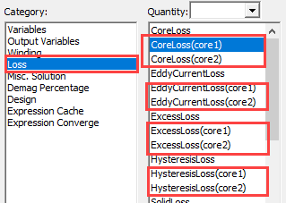
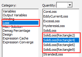
Select or clear Output per object solid loss. When this check box is selected, solid loss will be output for :
- The solid loss quantities of the objects selected in the Set Eddy Effects dialog will show in the reporter. (Objects selected should not belong to stranded winding or stranded conductor.)
- Coil objects in solid windings.
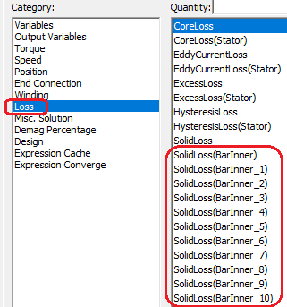
- For 2D designs:
  - Solid loss quantities of the coil objects assigned with the solid Current Excitation will show in the reporter.
  - Each bar in an end connection will be considered as a separate object for solid loss output.
  - All ring segments in one end-connection will be combined together as one virtual object for solid loss output.
    
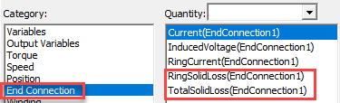
    If there are N end-connections (such as double cages), there will be N virtual objects.
Select or clear the Output error check box. When this check box is selected, the transient solver generates the output error data, which is then sent back to the desktop. The data can be viewed or used in the post processor, just as other transient solution data (such as power loss or winding).

Note: Output error is the percentage error in the total energy of the solution. This is a measure of the accuracy of the finite element approximation and can be used to judge if the mesh is good enough. Output error is calculated by finding the residual energy (the left-over energy calculated from the field after subtracting out the sources) divided by the total energy including the sources. Computing output error uses significant computation time.

For 3D Transient analysis only, select the desired Scalar Potential shape function: either Second Order (default), or First Order from the drop-down menu. You can also select the desired Scalar Potential on the Solver tab in the Properties window.

Use of the First Order scalar shape function, rather than the Second Order shape function, may be desirable for any of the following cases:
- If computational time is a main concern and solution accuracy is secondary. This might be useful for the initial design stage, before switching to using the more time consuming, and more accurate, second order scalar shape function.
- If the contour of the geometry is very complicated, it may not be possible to use the higher second order shape function due to the inability of relatively larger element size to properly represent the original geometry shape
- If the gradient of the magnetic field changes sharply, it may not be possible to use the higher second order shape function with large element size. Using a larger element size may not be able to adequately model the large change of material property with large element size, and nonlinear convergence may be difficult to achieve.
For 2D and 3D Transient designs, you can select the Number of Nonlinear Iterations check box. This provides an option for you to set both a Minimum iteration number to avoid non-converged solution, and a Maximum iteration number to avoid taking too much computation time. These values must be integers greater than 0. By default the values for Minimum and Maximum are 1 and 100, respectively. Maximum number should be greater than the Minimum number.
For 2D Transient analysis only, select the algorithm for the Time Integration Method using the drop-down menu.
- Backward Euler – Default
- Runge-Kutta – third-order algorithm for greater accuracy
Select or clear the Fast Reach check box.

For transient simulations whose winding excitations are an AC voltage source, the DC flux linkage component may take a very long time to decay, especially for a device with a large time constant. Selecting Fast Reach adds an additional voltage component to the original voltage definition during the first half-cycle to quickly eliminate the DC flux linkage, thus speeding up the solution process. You must also provide a Frequency of Added Voltage Source value that is greater than zero. The default value for Frequency of Added Voltage Source is 60 Hz. This frequency value is applied to all winding voltage sources.
Note:
- This speedup capability is only applicable to voltage sources whose integration of voltage quantity over one period is zero. This means the DC component of all voltage sources is zero.
- This feature is intended to be used in conjunction with windings of the type "voltage". If the winding is fed by an external circuit, a similar functionality is available using the alternating flux model defined in the properties of sinusoidal voltage sources. Alternatively, the dedicated AC_Model component can be applied if an external circuit is feeding the winding.
Select or clear the Auto Detect check box.

This option enables automatic detection of when steady state is reached based on a check of the flux linkage. When this option is selected, you must provide both a Frequency of Added Voltage Source value that is greater than zero (default value is 60 Hz), and a Stop criterion value that is greater than 0 and less than 1 (default value is 0.005). The smaller the Stop criterion value, the longer it will take to auto detect when steady-state is reached. For additional information on auto detect operation, refer to Automatic Detection of Reaching Steady State for Transient Simulations.

As needed for your design, select or clear settings in the Time Decomposition Method Option panel.

The Time Decomposition Method (TDM) is an HPC distributed analysis type based on domain decomposition along the time-axis, (rather than the normal geometry division) to parallelize the transient solution. Instead of solving Maxwell transient problems sequentially for each timestep, TDM enables timesteps to be solved simultaneously in parallel. Thus, TDM can be implemented on distributed memory parallel platforms based on MPI. TDM has very good scalability, resulting in significant speedup for both 2D and 3D transient solutions.

Note: Maxwell 3D A-Phi transient solver supports only General Transient TDM.

If you have enabled the Use Automatic Settings option in the Analysis Configuration dialog box, or if you have enabled the Transient Solver distribution type in the Analysis Configuration dialog box, you can select one of the following:

General Transient

For general transient (Non-Periodic) TDM applications, select General Transient. Using this method, TDM solves a collection of many timesteps simultaneously.

Periodic

TDM method intended for use in steady-state simulation. In such a case, all the setup and solutions at the first timestep will be the same as those at the last timestep of one period. Setup includes source, boundary, and position in electrical degrees. The solutions include all electrical and magnetic quantities. To use this method, all current in windings and all induced eddy currents in the conducting region should have the same time period. For example, an induction machine cannot be solved using the Periodic method because the time period of the currents in the stator winding is different from the time period of induced eddy current in the rotor bars.

Periodical TDM is computationally very efficient if a problem is applicable. But because all timesteps over one period have to be solved simultaneously (cannot be divided into subdivision as the case for general TDM transient), the memory requirement may prevent users from using periodical TDM. To this end, the support of half-periodical TDM is able to effectively cut memory usage to roughly half.

You can also select a Half-periodic option. This TDM option can cut your computer’s memory usage when solving Maxwell transient problems. If all physical quantities satisfy anti-periodic condition along Time axis, a problem can be solved using this option so that memory usage can be cut to almost half. Also, since the total timesteps to be solved are halved, the total computation time is also cut roughly by half.

For 2D designs, the Thermal Two-Way Coupling\Relaxation setting can be used to improve two-way coupling convergence by applying the relaxation factor to the temperature field. When the thermal modifier takes on a nonlinear form, the convergence of the solution field in Maxwell's equations may fail during two-way coupling iterations. With nonlinear iterations, using an under-relaxation factor can mitigate the risk of overshooting in the property updating process.

The range of the relaxation factor is from 0 to 1. In general, a smaller relaxation value helps convergence, but may increase the total number of iterations. The default relaxation factor is 1.0.

The Thermal Two-Way Coupling\Relaxation setting is applicable only when Enable Feedback is checked in Temperature of Objects window, which invokes two-way coupling instead of one-way coupling. The relaxation setting is

applicable to all Maxwell 2D designs,
applicable to both geometry modes (Cartesian XY and Cylindrical about Z),
does not support non-intrinsic and intrinsic variables.

If activated in the Solve Setup window, the Relaxation Factor is also available in the Solve Properties window: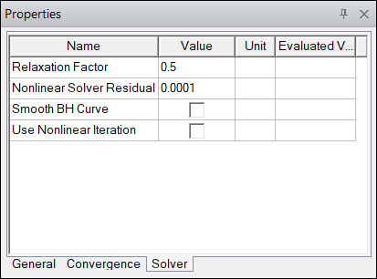

Defining Settings on the Solver Tab for Transient Solutions

Related Topics