Creeping Wave VRT Plots

This section describes how to use Visual Ray Trace (VRT) with Creeping Wave for Using Visual Ray Trace (VRT) with Creeping Wave for Antenna Placement and for Using Visual Ray Trace (VRT) with Creeping Wave for RCS.

Using Visual Ray Trace (VRT) with Creeping Wave for RCS

1. Once you have an appropriate HFSS design, there are three different ways in the user interface to create a new Visual Ray Trace Plot with Creeping Rays:

• Right-click the Field Overlays icon in the Project Tree and select Plot VRT...>Creeping Wave from the short cut menu.
• Right-click the 3D Modeler window and select Plot VRT...>Creeping Wave from the pop-up menu.
• Click HFSS>Fields>Plot VRT...>Creeping Wave

After you use one of these approaches, the Create Creeping Wave VRT Plot dialog displays:

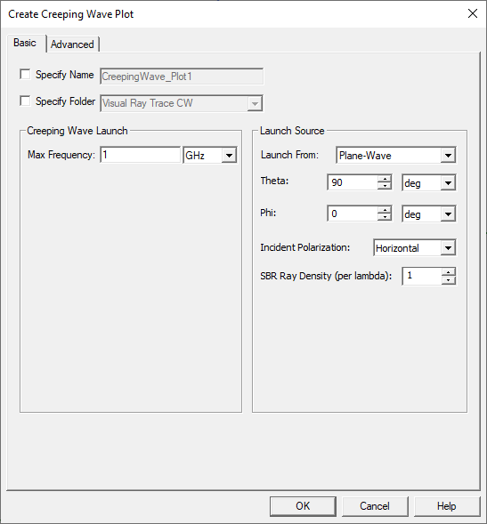
To Specify Name check the box to enable the text field. To Specify Folder, check the box to enable the selection menu.

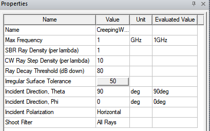
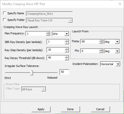
2. Set the Creeping Wave Ray Launch parameters

• Max Frequency should be set to the maximum frequency desired for the simulation. For simulations spanning multiple frequencies, the creeping wave settings should be tested at the highest simulation frequency.
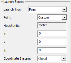
• Launch from parameters includes a menu for selecting the source as Plane-Wave or Point. For Plane-Wave, you specify the plane wave's incident direction by specifying Theta and Phi in spherical coordinates. If you select Point, the fields change to X, Y, and Z for a Global CS.
  
• Incident Polarization specifies the polarization of the incident plane wave as horizontal (Phi directed) or vertical (Theta directed). In conjunction with the Ray Decay Threshold setting, the choice of incident polarization differentially influences the propagation distance of individual creeping rays since their rate of decay depends on the polarization of their associated fields. In general, creeping rays launched from the shadow boundary where the incident electrical field is perpendicular to the surface decay more slowly than for those where the field is parallel to the surface.
• SBR Ray Density (per lambda) controls SBR ray density per lambda

Caution: The settings in this diagram are used by the VRT to test if the creeping waves are propagating as expected. These parameters are not automatically transferred to the Creeping Wave Settings for simulation. You need to set the simulation Creeping Wave Settings manually.

3. Optionally select the Advanced tab.
   

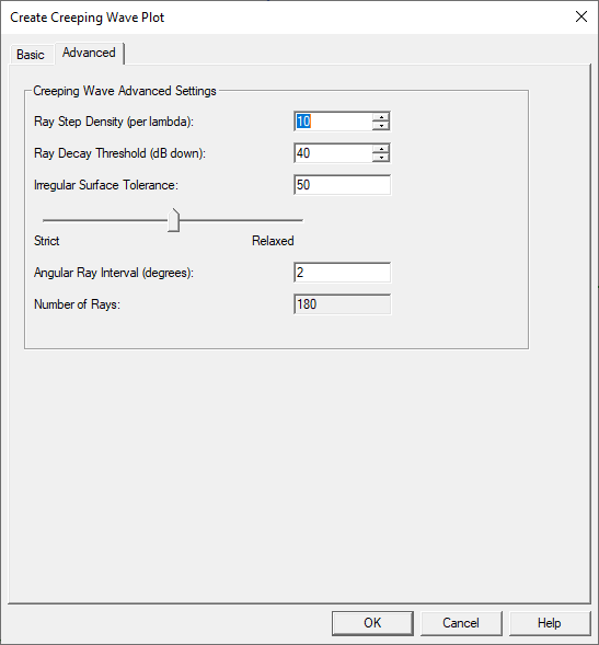
Ray Step Density (per lambda) controls lateral sampling along the direction of propagation along the surface.

Ray Decay Threshold controls how far the creeping rays propagate by terminating each ray once its power density decay (defined as dB down from its level at its starting point at the shadow boundary) exceeds this threshold.

Irregular Surface Tolerance is a single control for a collection of tolerances that determine creeping rays’ sensitivities to local surface irregularities that theoretically should block their further propagation. Moving the slider toward Relaxed allows creeping rays to propagate through small surface irregularities that may arise through defects in the input geometry or due to limitations of curvature extraction accuracy. However, setting this tolerance too relaxed may allow creeping waves to pass through concave surfaces, saddle surfaces, or wedges, which are not supported by creeping wave physics. The intention is that creeping rays only propagate over the convex portions of surfaces, and some user judgment is required in correctly setting the Irregular Surface Tolerance for each situation.

Angular Ray Interval (degrees) controls the density of rays that are generated along the nearest surface, starting under the current source, and spanning the 360 degrees around the current source.

Number of Rays indicates how many CW rays will be launched. This is a read-only field that is internally computed by dividing 360 degrees by the Angular Ray Interval

3. Click OK to dismiss the dialog to runs the VRT generation to produce SBR+ Creeping ray data. Only the geometries contained in the SBR+ regions are used for the VRT ray generation.
4. The “Shoot Filter” selections are disabled in the dialog box, and moved to the Visual Ray Trace CW folder properties as described below.
   

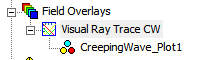
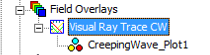
A new “Visual Ray Trace CW” plot folder is created under Field Overlays, which contains one or more “CreepingWave_Plot” items.

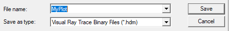
You can right-click on the VRT plot to display the Export Plot... command.

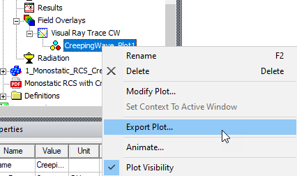
This allows you to export Visual Ray Trace Binary Files using a .hdm suffix.

If you run Plot VRT...>Creeping Wave again, that creates an additional CreepingWave_Plot item under the Visual Ray Trace CW folder, or a different folder name if you specify one in the Create Creeping Wave VRT Plot dialog.

Creeping Wave Plot Properties

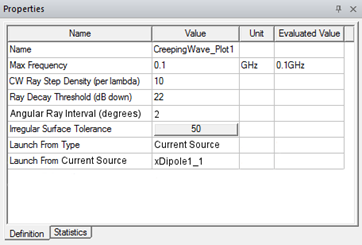
The Properties of each CreepingWave_Plotn item are the same as those created in the Create Creeping Wave VRT Plot dialog.

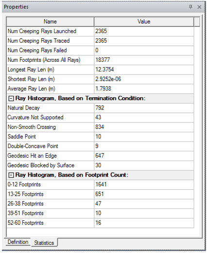
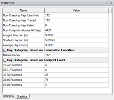
Each Creeping Wave plot has an additional read-only tabbed property page that displays Ray Statistics output from the ray generation process.

Modifying Creeping Wave Plots

You can modify Creeping Wave properties directly in the Properties window to cause immediate updates to the plot data. You can also right-click the plot item and select Modify Plot… to again bring up the Create VRT Plot dialog to make multiple changes and then commit them to the same, or a differently named plot.

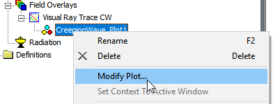
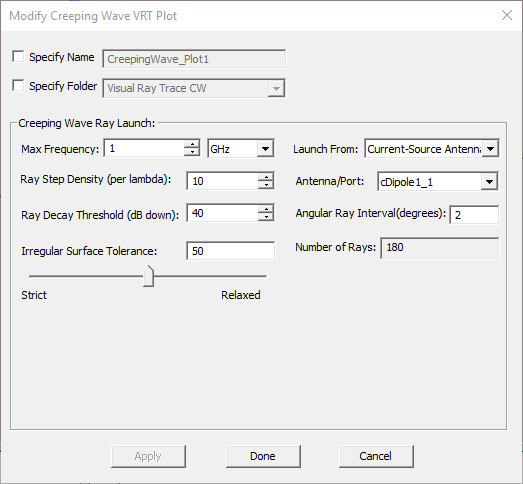
This opens a Modify Creeping Wave VRT Plot dialog.

Design Edits that Invalidate the Mesh Invalidate Creeping Ray VRT Plots

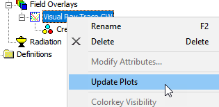
Any design edits that invalidate the mesh (geometry delete, modify, or change in boundary condition assignment) also invalidates VRT plots. HFSS does not automatically regenerate the VRT plot after a design edit. You can update plots update by right-clicking on the Visual Ray Trace SBR folder and selecting Update Plots.

Modification in SBR+ Wedge Setting parameters invalidates the VRT plot when “Shoot UTD Rays” is turned on.

In addition for UTD rays, a modification to the geometry and/or boundary condictions should automatically cause new SBR+ wedge to be generated whenever the VRT plot is manually updated.

Visual Ray Trace CW Folder Properties

All the render and filter parameters appear as Properties of the parent Visual Ray Trace CW folder. Each Visual Ray Trace CW plot folder provides a grouping of render/filter attributes. Much like setting specific plot attributes like 2D plot extents, scaling, colormaps, etc., the render and filter parameters for all VRT plots are performed at this folder level. The different categories of render and filter operations are kept as separate tabs for: Rendering and Filters.

All render and filter property changes are immediate and will automatically refresh the 3D modeler window

Rendering Properties Tab

The Rendering tab properties control which items are drawn for each ray track, as well as width and shadow boundary controls:

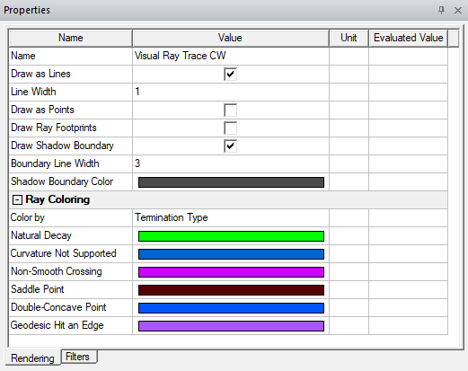
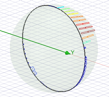
• Draw as Lines: show the “rays” connecting the launch point, each intersection point, and the exit point.
• Draw as Points: show the point for each ray bounce where we intersect the geometry.
• Draw Ray Footprints: show the ray tube projection for each ray bounce.
  
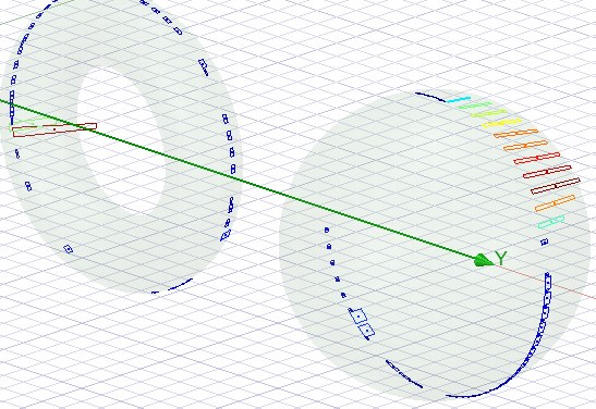
• Draw Shadow Boundary: shows the edge that defines the shadow region.
  
  

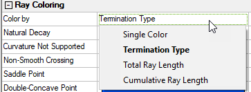
Ray Coloring controls:

• Color by: Can be Single Color, Termination Type, Total Ray Length, or Cumulative Ray Length.
  
  
• If you select Termination Type, the terminations listed depend on those generated by the plot.
• If you select Single Color, the properties are Line Color, Point Color, and Footprint Color.
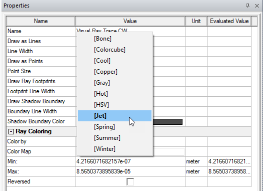
• If you select Total Ray Length or Cumulative Ray Length, the properties are Color Map (which offers many choices, shown below), Min, Max, and Reversed.
  

Filter Properties Tab

The Filter properties tab controls which ray tracks and/or bounces are shown in the 3D modeler window. Filter by Launch Angle is unique to CW for antennas (vs. CW for RCS).

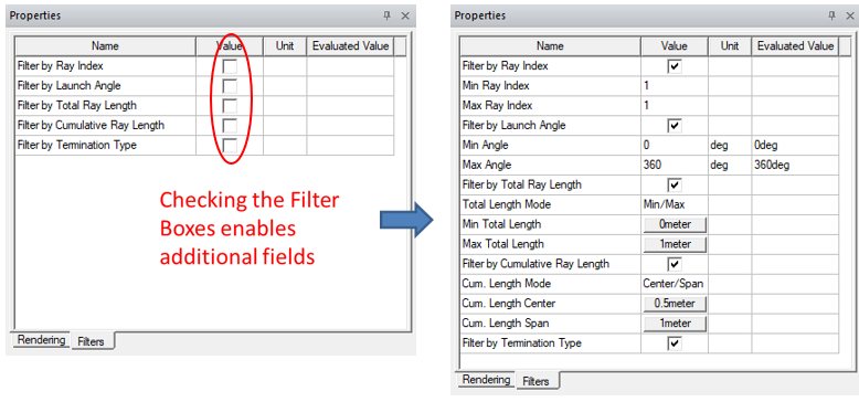
Selecting any of Ray Index, Launch Angle, Total Ray Length, opens Min and Max parameters for that filter.

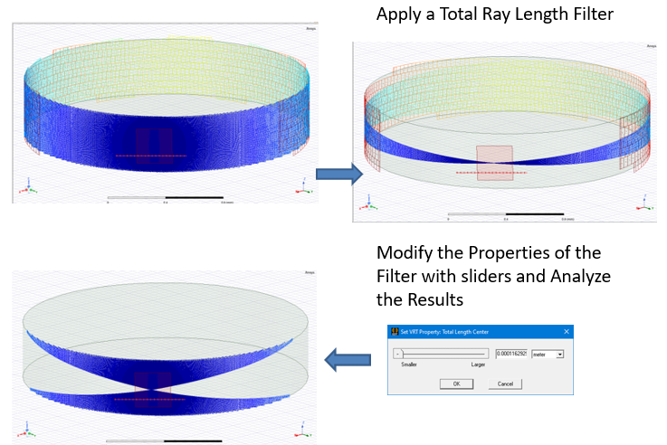
Filter By Total Ray Length: use Total Length Mode of either Center/Span or Min/Max. You can assign length values as a variable. Using a variable permits you to creating an animation by sweeping the variable.

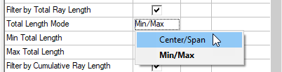
Selecting Center/Span enables buttons for Total Length Center and Total Length Span. Clicking one of these buttons opens Slider window that allows you to modify the filter values and see in real-time the changing rays in the model view window.

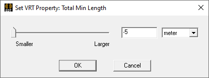
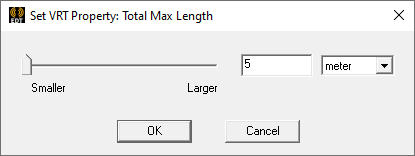
Selecting Min/Max enables buttons for Total Min Length and Total Max Length. Clicking a button opens a Slider window for real time control of the modeler window.

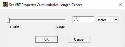
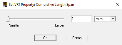
Filter By Cumulative Ray Length: use with the Center/Span or Min/Max selections. You can assign length variables as the value. Using a variable allows you to animate the plot by sweeping that variable. Selecting Center/Span enables buttons for Cumulative Length Center and Cumulative Length Span. Clicking one of these buttons opens Slider window that allows you to modify the filter values and see in real-time the changing rays in the model view window.

Selecting Min/Max enables buttons for Cumulative Length Center and Cumulative Length Span. Clicking a button opens a Slider window for real time control of the modeler window.

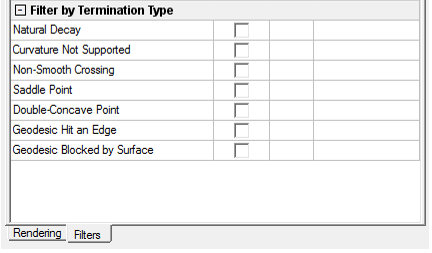
Selecting Filter by Termination Type lists the terminations available in the model.

Using Visual Ray Trace (VRT) with Creeping Wave for Antenna Placement

1. Once you have an appropriate HFSS design, there are three different ways in the user interface to create a new Visual Ray Trace Plot with Creeping Rays:

• Right-click the Field Overlays icon in the Project Tree and select Plot VRT...>Creeping Wave from the short cut menu.
• Right-click the 3D Modeler window and select Plot VRT...>Creeping Wave from the pop-up menu.
• Click HFSS>Fields>Plot VRT...>Creeping Wave

After you use one of these approaches, the Create Creeping Wave VRT Plot dialog displays.

From the Launch From: drop down menu, select the Current-Source antenna source and then select the desired Antenna/Port for launching creeping waves. This will change some dialog fields, from the Plane Wave configuration, as follows.

To Specify Name check the box to enable the text field. To Specify Folder, check the box to enable the selection menu.

2. Set the Creeping Wave Ray Launch parameters

• Max Frequency should be set to the maximum frequency desired for the simulation. For simulations spanning multiple frequencies, the creeping wave settings should be tested at the highest simulation frequency.
• Ray Step Density (per lambda) controls longitudinal sample along the direction of propagation along the surface.
• Ray Decay Threshold controls how far the creeping rays propagate by terminating each ray once its power density decay (defined as dB down from its level at its starting point at the shadow boundary) exceeds this threshold.
• Irregular Surface Tolerance is a single control for a collection of tolerances that determine creeping rays’ sensitivities to local surface irregularities that theoretically should block their further propagation. Moving the slider toward Relaxed allows creeping rays to propagate through small surface irregularities that may arise through defects in the input geometry or due to limitations of curvature extraction accuracy. However, setting this tolerance too relaxed may allow creeping waves to pass through concave surfaces, saddle surfaces, or wedges, which are not supported by creeping wave physics. The intention is that creeping rays only propagate over the convex portions of surfaces, and some user judgment is required in correctly setting the Irregular Surface Tolerance for each situation.
• Launch from parameters includes a menu for selecting the source for Antenna placement Creeping Wave, the near field parametric antenna or Near Field link you specified.
• Antenna /Port lists available antennas/ports that can be represented by current sources.
• Angular Ray Interval (degrees) controls the density of rays that are generated along the nearest surface, starting under the current source, and spanning the 360 degrees around the current source
• Number of Rays indicates how many CW rays will be launched. This is a read-only field that is internally computed by dividing 360 degrees by the Angular Ray Interval.

Caution: The settings in this diagram are used by the VRT to test if the creeping waves are propagating as expected. These parameters are not automatically transferred to the Creeping Wave Settings for simulation. You need to set the simulation Creeping Wave Settings manually.

3. Click Done to dismiss the dialog and run the VRT generation to produce SBR+ Creeping ray data. Only the geometries contained in the SBR+ regions are used for the VRT ray generation.
4. The “Shoot Filter” selections are disabled in the dialog box, and moved to the Visual Ray Trace CW folder properties as described below.
5. After the plot is generated, you can use the plot properties to update or change the appearance of the plot.
   

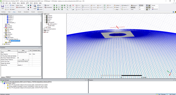
A new “Visual Ray Trace CW” plot folder is created under Field Overlays, which contains one or more “CreepingWave_Plot” items.

If you run Plot VRT...>Creeping Wave again, that creates an additional CreepingWave_Plot item under the Visual Ray Trace CW folder, or a different folder name if you specify one in the Create Creeping Wave VRT Plot dialog.

Creeping Wave Plot Properties

The Properties of each CreepingWave_Plotn item are the same as those created in the Create Creeping Wave VRT Plot dialog.

Each Creeping Wave plot has an additional read-only tabbed property page that displays Ray Statistics output from the ray generation process.

Modifying Creeping Wave Plots

You can modify Creeping Wave properties directly in the Properties window to cause immediate updates to the plot data. You can also right-click the plot item and select Modify Plot… to again bring up the Create VRT Plot dialog to make multiple changes and then commit them to the same, or a differently named plot.

This opens a Modify Creeping Wave VRT Plot dialog.

Design Edits that Invalidate the Mesh Invalidate Creeping Ray VRT Plots

Any design edits that invalidate the mesh (geometry delete, modify, or change in boundary condition assignment) also invalidates VRT plots. HFSS does not automatically regenerate the VRT plot after a design edit. You can update plots update by right-clicking on the Visual Ray Trace SBR folder and selecting Update Plots.

Visual Ray Trace CW Folder Properties

All the render and filter parameters appear as Properties of the parent Visual Ray Trace CW folder. Each Visual Ray Trace CW plot folder provides a grouping of render/filter attributes. Much like setting specific plot attributes like 2D plot extents, scaling, colormaps, etc., the render and filter parameters for all VRT plots are performed at this folder level. The different categories of render and filter operations are kept as separate tabs for: Rendering and Filters.

All render and filter property changes are immediate and will automatically refresh the 3D modeler window

Rendering Properties Tab

To change the render and filter settings applied to the VRT plot, the plot folder containing the plot item may be selected to access the Plot Folder properties for all plots contained in the folder.

The Rendering tab properties control which items are drawn for each ray track, as well as width and shadow boundary controls:

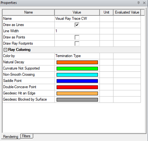
Render properties include being able to select display of lines, points, and footprints, and with Color-by options for Single Color, Termination Type, Total Ray Length, and Cumulative Ray Length.

Ray Coloring controls:

• Color by: Can be Single Color, Termination Type, Total Ray Length, or Cumulative Ray Length.
  
  
• If you select Termination Type, the terminations listed depend on those generated by the plot.
• If you select Single Color, the properties are Line Color, Point Color, and Footprint Color.
• If you select Total Ray Length or Cumulative Ray Length, the properties are Color Map (which offers many choices, shown below), Min, Max, and Reversed.
  

Filter Properties Tab

The Filter properties tab controls which ray tracks and/or bounces are shown in the 3D modeler window. Filter by Launch Angle is unique to CW for antennas (vs. CW for RCS).

Selecting any of Launch Angle, Total Ray Length, Cumulative Ray Length opens Min and Max parameters for that filter. Selecting Termination Type lists the terminations available in the model.