Near Field Analysis using Incident Plane Wave in SBR+ Design

SBR+ designs and HFSS designs with SBR+ Hybrid regions can provide near field analysis and overlay rectangular near field plots on the modeler window. For SBR+, the near field setup must be defined before simulation, as is currently done for an SBR+ far field setup. The near field setups allow for a 3-D grid of sample points to be defined.

This chapter describes the process flows for Near Field Analysis using Incident Plane Wave in SBR+ designs, and for HFSS Terminal or Modal designs with SBR+ Hybrid Regions.

Prerequisites

• Create an HFSS design with SBR+ regions, either driven model or terminal solution type or an SBR+ solution type.
• Near Field analysis with SBR+ supports antenna port excitations and supports Incident Plane wave sources.
• You must specify Tx or Tx/Rx roles for antenna ports, or Incident Plane wave source to make Near Field analysis available.
• Note: When there are any encrypted components in the design, Near Field Analysis will be aborted.

Technical Notes

• Placing near-field observation points very close to an SBR+ region surface can increase SBR+ simulation time, sometimes significantly; when a near-field observation point is near an SBR ray footprint, the solver needs to finely subdivide the ray footprint to maintain accuracy in its scattered field contribution to that observation point."

• In the SBR+ methodology, final (total) field results are always coherently assembled upon the base of an incident field from the source radiation radiating in free space. That means the fields start strong everywhere before the SBR rays are launched. Any reduction of this initial field due to structural blockage is achieved through destructive interference with a comparably strong scattered field arising from SBR currents painted by the rays hitting the blocking structure.

  Under conditions of strong shadowing, as in the extreme example of volume enclosed by a metal surface, one expects very weak or zero fields in the shadowed region. Destructive interference is rarely perfect, and one can generally expect some finite field at every near-field observation point. Field extinction (or nulling) in an enclosed volume is only achieved to the extent of predicting currents with high fidelity upon the enclosing surface. If you observe unrealistically large fields in a deeply shadowed or enclosed region, try increasing SBR Ray Density until the results converge. You can also try deploying SBR+ physics enhancements, such as UTD Edge Diffraction Rays and, if the source is an antenna mounted on a smooth metal surface with convex curvature, Creeping Rays. However, SBR+ remains an asymptotic (high-frequency) approximation best suited for electrically large scattering geometry, so the accuracy of painted currents and therefore field extinction in shadowed spatial regions is ultimately limited by the accuracy of multi-bounce geometric optics (GO), UTD edge diffraction, and UTD creeping-wave formulations.

Process Flow for Near Field Analysis in SBR+ Design

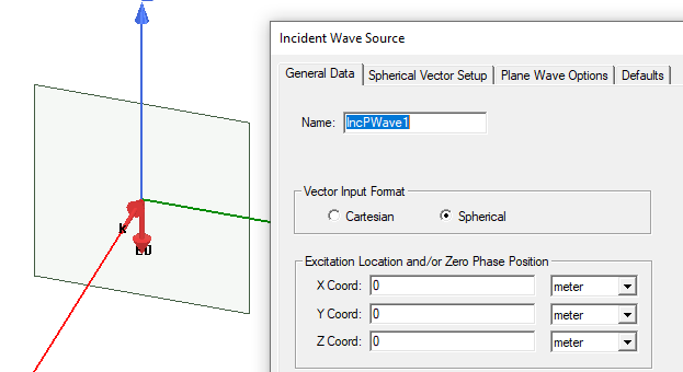
1. For this design with SBR+ solution type, create an Incident Plane Wave as the example below shows.
   
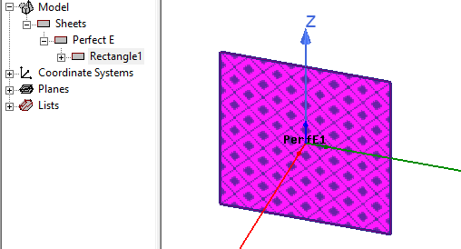
2. Add scene geometry components. This example contains a rectangle assigned a Perfect E boundaries.

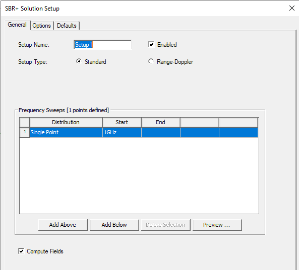
3. Right-click on the Analysis icon in the Project tree and select Add Solution Setup..., or select the Simulation tab of the ribbon and select the Setup icon.

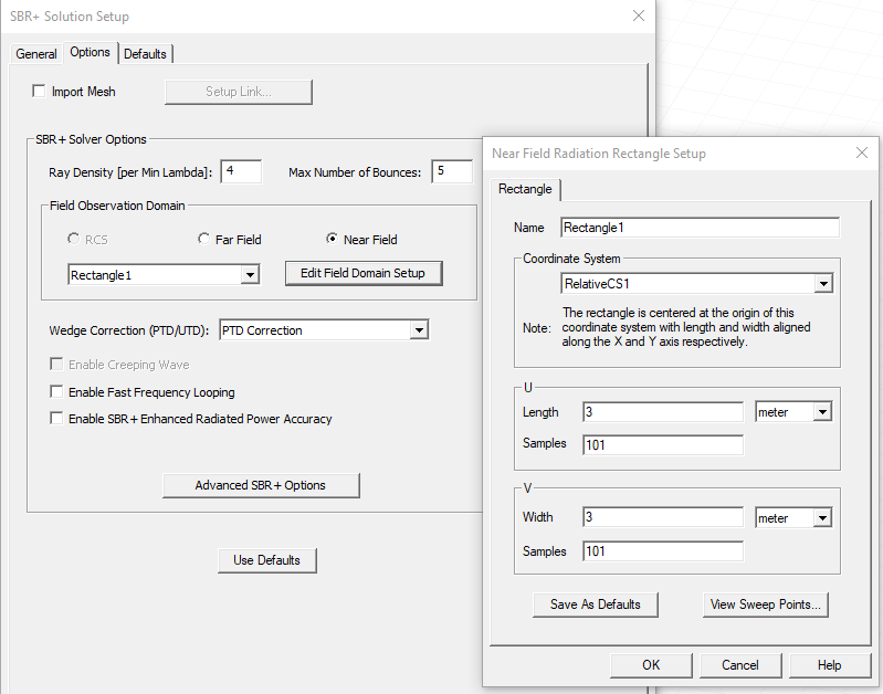
The SBR+ Solution Setup dialog displays. On the General tab check the box to Compute Fields.

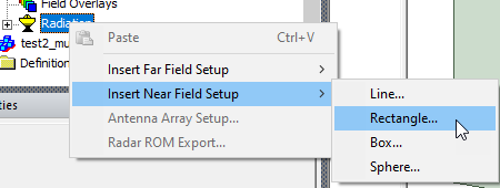
4. Next we need to create a Near Field observation domain (a Near Field Radiation Setup) and assign it to the solution setup. Right-click on the Radiation icon in the Project tree and select Insert Near Field Setups> and select Rectangle... from the menu.

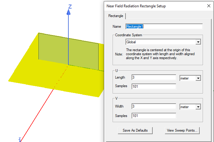
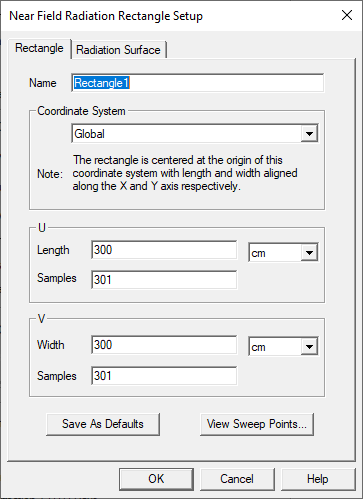
This opens a Near Field Radiation Rectangle Setup dialog box. You specify the name, Coordinate System, U and V length, units, and number of samples. To move or re-oriented the near-field sampling grid, set the Coordinate System to one with the desired translation and rotation, first creating a new coordinate system for this purpose if needed. This first example shows a setup based on the Global Coordinate system.

Returning to the Analysis Setup dialog box, the Options tab contains the Field Observation Domain configuration. Any Near Field or Far Field setups that you create, or that exist for the design, are listed in the Field Observation Domain drop down menu of Options tab of the SBR+ Solution Setup.

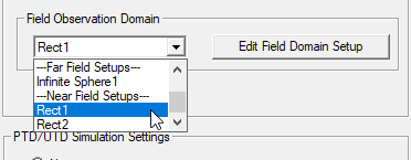
The Field Observation Domain drop down menu can also be used to directly create a new domain by selecting "Create Near Field..." The setup dialog for the Near Field Radiation Rectangle is then used to create/configure the Rectangle. Closing the dialog returns to the Analysis setup. This is made available as a shortcut, so note that the full set of Near Field Radiation setups is not available here. Those setups (Box, Line, etc.) can be created via the Radiation object in the Project tree as previously described. Note this example also assigns PTD Correction to include diffraction of the sharp plate edges in the simulation.

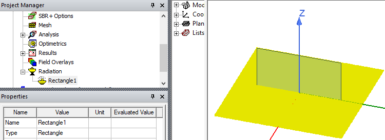
5. To visualize the sample points in the Modeler window, select the Radiation setup in the Project tree.

6. Right click on the Solution setup icon the Project tree and click Analyze to run the simulation.
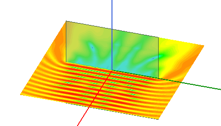
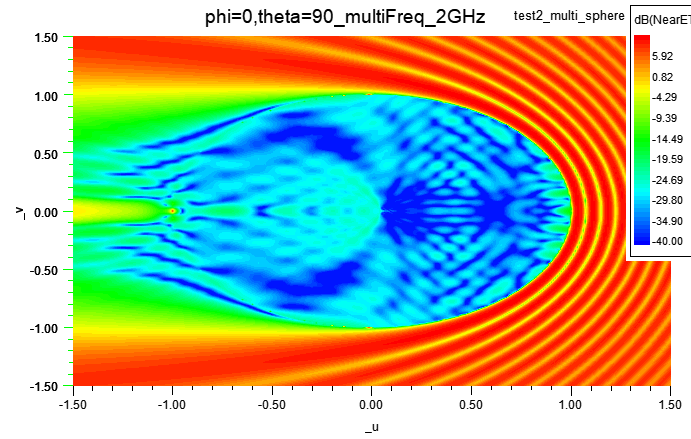
7. Generate a Rectangular Contour Plot of the Near Field.

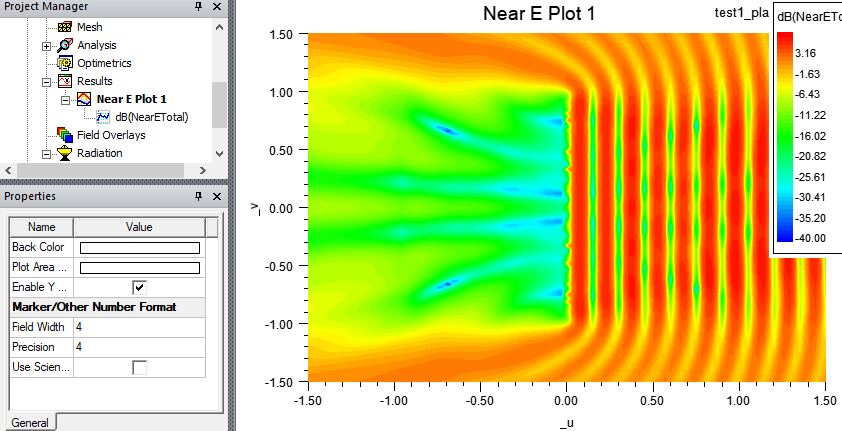
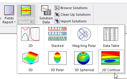
Right-click on the Results icon in the Project tree and select Results>Create Near Fields Report...>Rectangular Contour Plot, or select the Results tab of the ribbon, and click on the Near Fields Report icon and select the 2D Contour icon. These bring up the Reporter dialog.

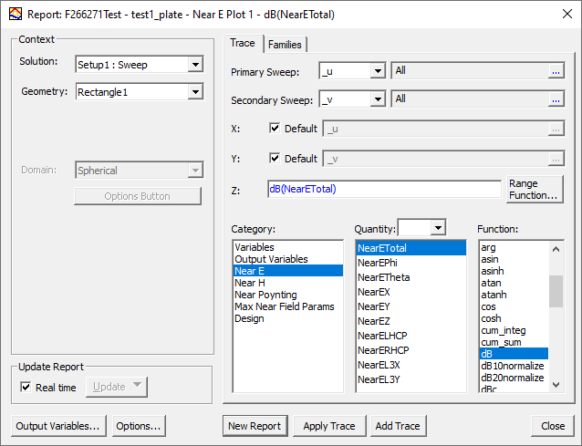
Select the Near Field radiation Rectangle1 as the for the Context. Select Near E as the Category, NearETotal as the Quantity, and dB as the Function., and click New Report. This creates the Near E Rectangular Contour plot.

Note that these plots are associated with the local coordinate system for positions and global coordinate system for field polarizations. Point positions of Sweeps _u and _v are associated with X and Y of the local Relative CS in which the near-field sample points are defined, while the reported polarized field components are associated with the orientation of the global coordinate system. For example, suppose we define the Relative CS, named Rect2, for the Rect2 grid is rotated by theta = -90 deg around the Y axis of global coordinates. Thus, the near-field sample points are located in the XY plane of Rect2 Relative CS and also in the YZ plane of global coordinates. Point positions of the sweep _u are associated with the X axis of the local coordinate system, which is the Z axis of the global coordinate system. On the other hand, selecting NearEZ in a field report will show the electric field component oriented along the Z axis of global coordinates, not the Z axis of the Rect2 RelativeCS. It is important to understand that the designated field polarizations are always oriented according to global coordinates.

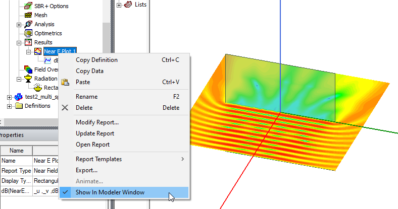
8. To overlay the near field report contour plot in Model window, right click on the Plot in the Project tree and select Show in Modeler Window.

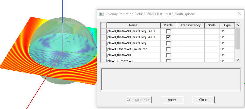
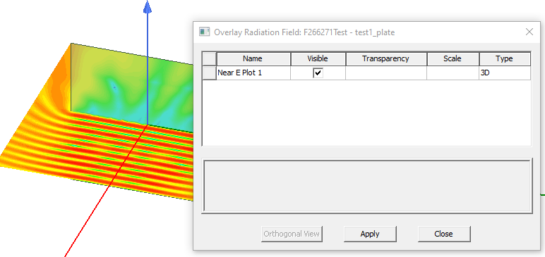
You can also right click in the Modeler window and select Plot Fields...>Radiation Field... to open the Overlay Radiation Field dialog box, and check for the plot to be visible. If more than one plot exists, you can overlay any or all of them that have current solution data.

Process Flow for Near Field Analysis in HFSS Modal or Terminal Design with SBR+ Hybrid Regions

1. Create an HFSS design of HFSS with Hybrid and Arrays solution type as either Modal or Terminal.
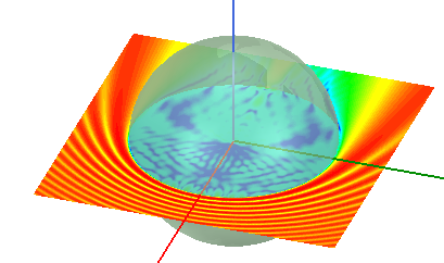
2. Add scene geometry components. For this example, we add a copper sphere.
   
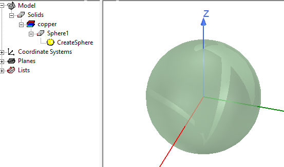
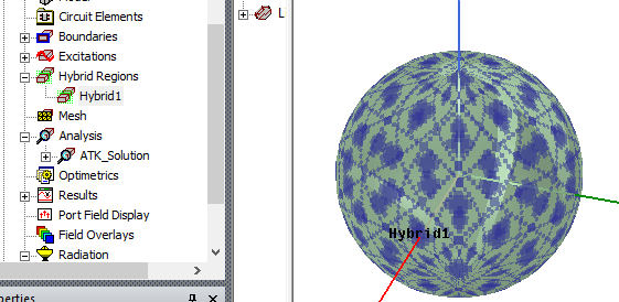
3. Assign SBR+ hybrid region(s). In this example, assign the and SBR+ Hybrid Region to the sphere.
   
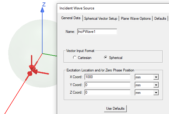
4. Add an Incident Plane Wave source excitation.
   
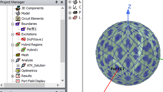
5. For driven Modal/Terminal solution types, the antenna geometries with the excitation must be surrounded by a FE-BI, a Radiation boundary, or a Perfect E boundary. In this example, we assign the sphere a Perfect E boundary.
   
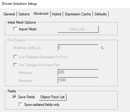
6. Add an Analysis Setup.

On the Advanced tab check the box to Save Fields.

On the Hybrid tab, select a Field Observation Domain by clicking on the dropdown list and selecting Create Near Field... (or select an existing one, if already exists).

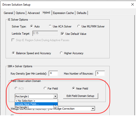
In this example, we Enable Creeping Wave. In the dialog to create the Rectangle setup, enter the desired parameters.

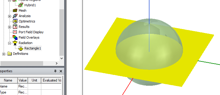
Select the newly created Radiation setup in the project tree to visualize the sample points in the 3D model window.

7. Run simulation
8. Generate a Rectangular Contour Plot of the Near Field.

Select Results>Create Near Fields Report...>Rectangular Contour Plot to bring up the Reporter dialog box, or on the Results tab of the ribbon, select 2D Contour form the Near Fields Report drop down.

In the Report dialog box, select the Near Field radiation setup for the report Context, and the desired Quantity and Function.

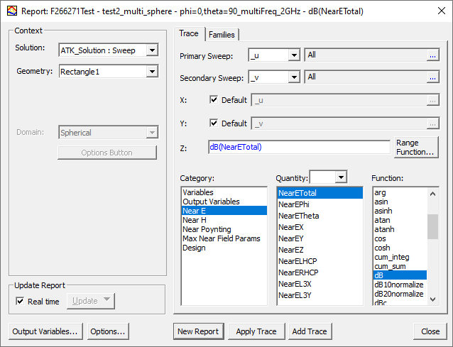
Select the Near Field radiation Field Observation Domain as the Geometry for the Context. Select Near E as the Category, NearETotal as the Quantity, and dB as the Function., and click New Report. This creates the Near E Rectangular Contour plot.

Be aware of that the point locations will be defined relative to the _u (X) and _v (Y) axes of the local relative coordinate system while the reported polarized field components are always aligned with global coordinates.

9. To overlay the near field report contour plot in Model window, right click on the Plot in the Project tree and select Show in Modeler Window.

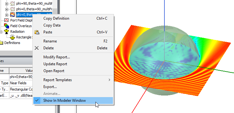
You can also right click in the Modeler window and select Plot Fields...>Radiation Field... to open the Overlay Radiation Field dialog box, and check for the plot to be visible. If more than one plot exists, you can overlay any or all of them that have current solution data.