Chapter 19: Effusion Cooling simulation in a 3D model Combustor

This tutorial is divided into the following sections:

19.1. Introduction

This tutorial demonstrates the process to set up perforated wall model and its capability for effusion cooling in a model combustor.

A slice of cylindrical combustor burning liquid fuel with methane () as the evaporated gas in hot air is studied using the FGM model in Ansys Fluent.

This tutorial demonstrates how to do the following:

Enable physical models, select material properties, and define boundary conditions for a turbulent combustion flow with FGM model.
Set up perforated wall to model effusion cooling effects.
Initiate and solve the combustion simulation using the pressure-based solver.
Examine the reacting flow results using graphics.

19.2. Prerequisites

This tutorial is written with the assumption that you have completed the introductory tutorials found in this manual and that you are familiar with the Ansys Fluent outline view and ribbon structure. Some steps in the setup and solution procedure will not be shown explicitly.

To learn more about turbulent combustion modeling and perforated walls, see the Fluent User's Guide and the Fluent Theory Guide.

19.3. Problem Description

The 3D model gas turbine combustor considered in this tutorial is shown in Figure 19.1: 3D model gas turbine combustor with liquid fuel Combustion of Methane. The flame considered is a turbulent diffusion flame with fuel supplied by liquid droplets. The air is introduced from the inlet with mass flow rate 0.10962 kg/s. Air flow is split into two streams, one goes through a swirl after which air and evaporated fuel mixed, and the other goes into the shroud. The fuel droplets are injected after the swirl and evaporation will occur. The evaporated fuel is set to be methane. After air and fuel are mixed, the flame is established in the main combustion chamber.

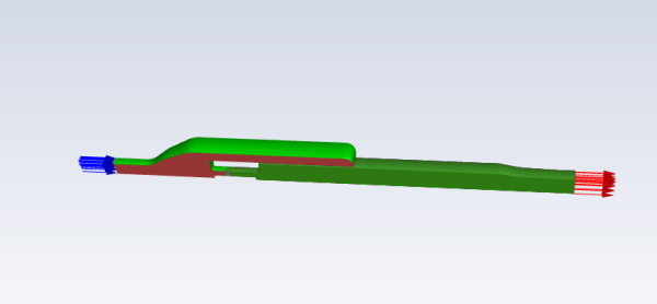
Figure 19.1: 3D model gas turbine combustor with liquid fuel Combustion of Methane

19.4. Background

In this tutorial, you will use the FGM turbulent combustion model and DPM model to simulate analyze the methane-air combustion system. The effusion cooling effects are modeled with perforated wall capability. The effusion cooling mass flow rate are determined by the pressure difference between the shroud and the main combustion chamber.

19.5. Setup and Solution

The following sections describe the setup and solution steps for this tutorial:

19.5.1. Preparation

To prepare for running this tutorial:

Download the effusion_cooling.zip file here .
Unzip effusion_cooling.zip to your working directory.
The SpaceClaim CAD file combustor_effusion.scdoc can be found in the folder.
Use the Fluent Launcher to start Ansys Fluent.
Select Meshing in the top-left selection list to start Fluent in Meshing Mode.
Select 3D under Dimension.
Enable Double Precision under Options.
Set Meshing Processes and Solver Processes to 4 under Parallel (Local Machine).

19.5.2. Meshing Workflow

Start the meshing workflow.
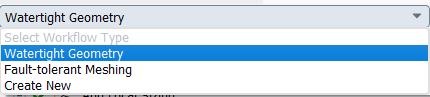
1. In the Workflow tab, select the Watertight Geometry workflow.
2. Review the tasks of the workflow.
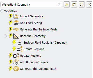
  Each task is designated with an icon indicating its state (for example, as complete, incomplete, etc. For more information, see Understanding Task States in the Fluent User's Guide). All tasks are initially incomplete and you proceed through the workflow completing all tasks. Additional tasks are also available for the workflow. For more information, see Customizing Workflows in the Fluent User's Guide.
Import the CAD geometry (combustor_effusion.scdoc).
1. Select the Import Geometry task.
2. For Units, select mm.
3. For File Name, enter the path and file name for the CAD geometry that you want to import (combustor_effusion.scdoc).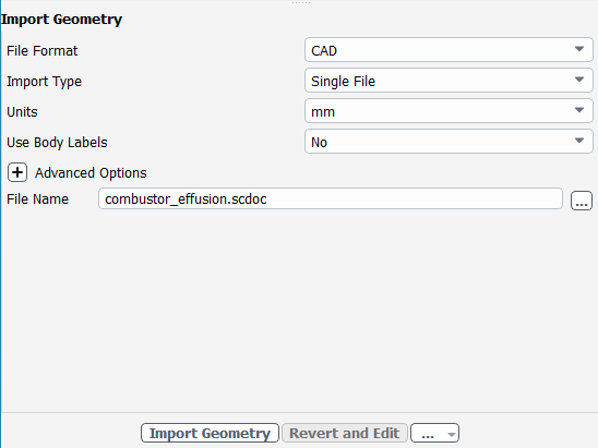
  Note: The workflow only supports *.scdoc (SpaceClaim), Workbench (.agdb), and the intermediary *.pmdb file formats.
4. Click Import Geometry.
  This will update the task, display the geometry in the graphics window and allow you to proceed onto the next task in the workflow.
  Figure 19.2: The Imported CAD Geometry for the Combustor
  
  The combustor geometry has been enclosed in a suitable flow domain, which should provide distinct regions of inflow and outflow for a range of angles of attack, and avoids having the bow shock that forms in such flows from contacting the inflow surfaces..
  Note: Alternatively, the ... button next to File Name can be used to locate the CAD geometry file, after which, the Import Geometry task automatically updates, displaying the geometry in the graphics window, and the workflow automatically progresses to the next task.
  Throughout the workflow, you are able to return to a task and change its settings using either the Edit button, or the Revert and Edit button.
Add local sizing.
Local mesh sizing controls are added on the liner surfaces using face sizing.
1. In the Add Local Sizing task, add local sizing controls to the faceted geometry by selecting yes:
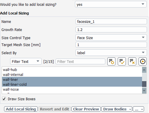
  In this tutorial, we will add local sizing around the surfaces of the liner, since they are areas where we require a more refined mesh.
  1. At the prompt for adding local sizing, select yes.
  2. Retain the default facesize_1 for the Name of the size control.
  3. Specify 1.2 for the Growth Rate.
  4. Retain Face Size for the Size Control Type.
  5. Specify 1 for the Target Mesh Size.
  6. Select Label for the Select By.
  7. Select wall-liner and wall-liner-cold.
  8. Click Add Local Sizing.
Generate the surface mesh.
With the local sizing set as described above, the global surface mesh sizing only defines the largest elements on other surfaces.
1. In the Generate the Surface Mesh task, you can set various properties of the surface mesh for the faceted geometry.
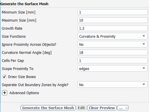
2. Specify 1 for the Minimum Size.
3. Specify 10 for the Maximum Size.
  Note: The red boxes displayed on the geometry in the graphics window are a graphical representation of size settings. These boxes change size as the values change, and they can be hidden by using the Clear Preview button.
4. Specify 1.2 for the Growth Rate.
5. Click Generate the Surface Mesh to complete this task and proceed to the next task in the workflow.
Describe the geometry.
When you select the Describe Geometry task, you are prompted with questions relating to the nature of the imported geometry.
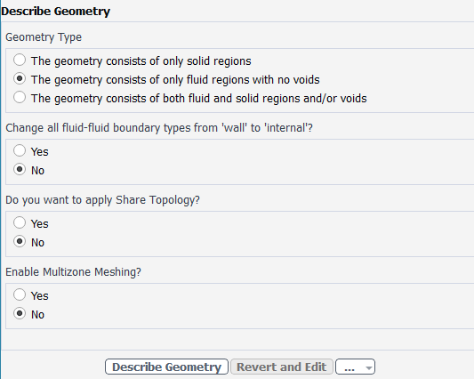
1. Select The geometry consists of only fluid regions with no voids option under Geometry Type, since this model contains only the fluid region.
2. Keep the rest of the default settings for this task.
3. Click Describe Geometry to complete this task and proceed to the next task in the workflow.
Confirm and update the boundaries.
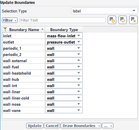
1. Select the Update Boundaries task, where you can inspect the mesh boundaries and confirm and change any designated boundaries accordingly. Ansys Fluent attempts to determine the correct arrangement of boundaries automatically.
2. Rename wall-internal to wall-int for the boundary name.
3. Rename Inlet-fuel to wall-fuel for the boundary name.
4. Select wall for the wall-fuel boundary type.
5. Select mass-flow-inlet for the inlet boundary type.
6. Click Update Boundaries and proceed to the next task.
Insert a new task and create the periodic boundaries.
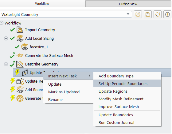
Right click on the Update Boundaries task, Insert New Task and select Set Up Periodic Boundaries.
1. Retain the default Select the Update Boundaries task, where you can inspect the mesh boundaries and confirm and change any designated boundaries accordingly. Ansys Fluent attempts to determine the correct arrangement of boundaries automatically.
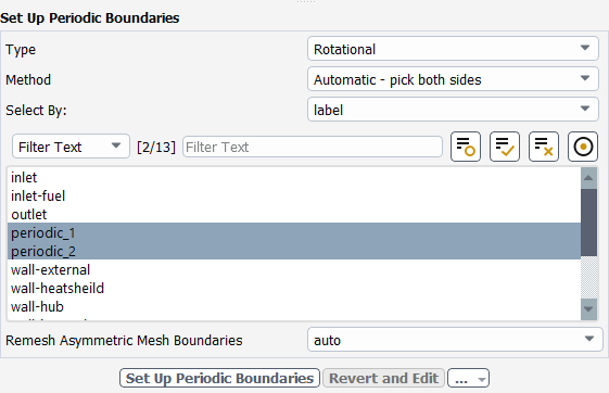
2. Retain the default Rotational for the Type of periodic boundary, Automatic - pick both sides for the Method and Label for Select By:.
3. Select periodic_1 and periodic_2 for the two sides of the periodic boundary.
4. Click Set Up Periodic Boundaries and proceed to the next task.
Update your regions.
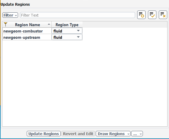
1. Select the Update Regions task, where you can review and change the tabulated names and types of the various regions that have been generated from your imported geometry and change them as needed.
2. The proposed region type is correct, so click Update Regions to update your settings.
Add boundary layers.
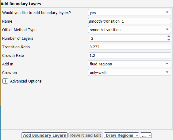
1. Select the Add Boundary Layers task, where you can set properties of the boundary layer mesh.
  For the Add Boundary Layers task, ensure yes is selected at the prompt as to define boundary layer settings. In this task, you can define specific details for capturing the boundary layer in and around your geometry.
2. Click Add Boundary Layers.
Generating the volume mesh.
With the local sizing set as described above, including bodies of influence, the global volume mesh sizing only defines the largest elements in the flow domain. In this case, the maximum is set to be consistent with the specified global surface mesh sizing.
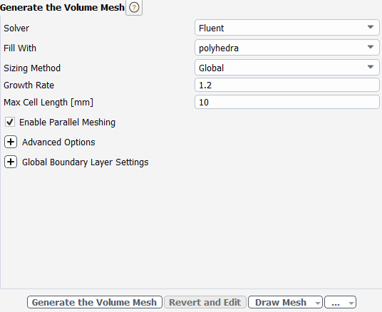
1. Select the Generate the Volume Mesh task, to set properties of the volume mesh.
2. Select the polyhedra for Fill With.
3. Specify 10 for Max Cell Length.
4. Retain the default selection of Enable Parallel Meshing.
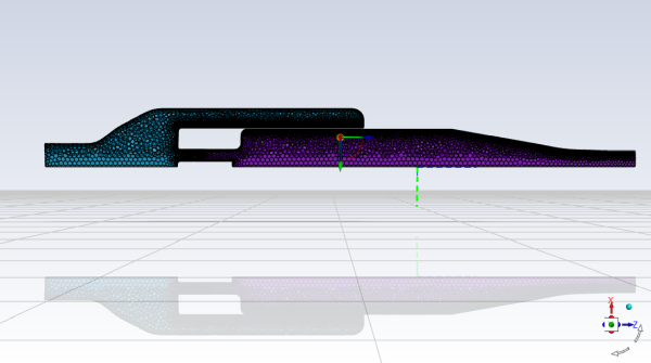
5. Click Generate the Volume Mesh.
  Ansys Fluent will apply your settings and proceed to generate a volume mesh for the geometry.. The mesh is displayed in the graphics window and a clipping plane is automatically inserted with a layer of cells drawn so that you can quickly see the details of the volume mesh.
Check the mesh.
Mesh → Check → Perform Mesh Check
Save the mesh file (combustor_effusion.msh.h5).
File → Write → Mesh...
Switch to Solution mode.
Now that a mesh has been generated using Ansys Fluent in meshing mode, you can now switch to solver mode to complete the set up of the simulation. Note that to obtain more accurate solutions a higher quality mesh should be used.
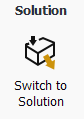
We have just checked the mesh, so select Yes when prompted to switch to solution mode.

19.5.3. Mesh

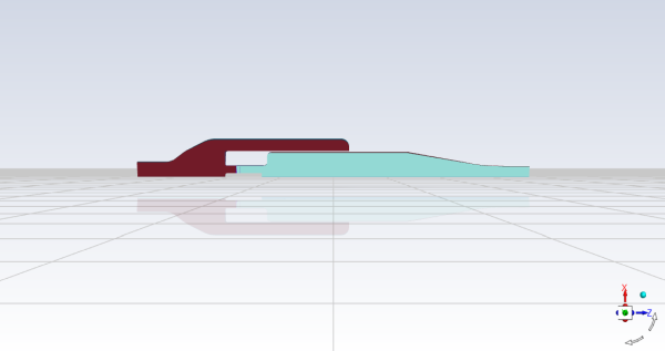
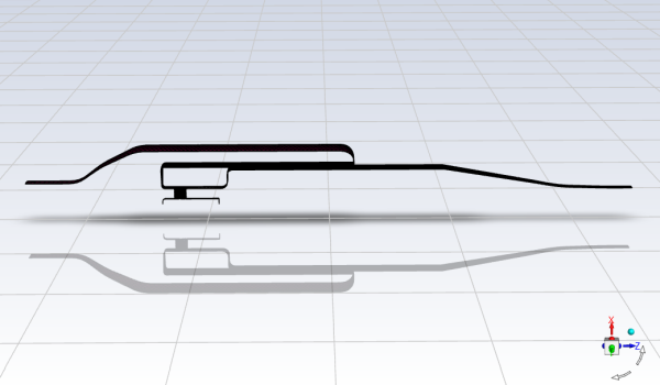
Examine the mesh.
Domain → Mesh → Display...
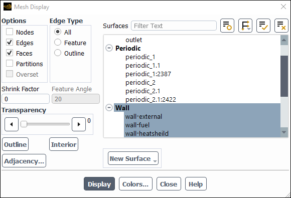
1. Enable Edges in the Options group box.
2. Ensure All is selected in the Edge Type group box.
3. Select Wall from the Surfaces selection list.
4. Click Display and close the Mesh Display dialog box.

19.5.4. Setting Up Physics

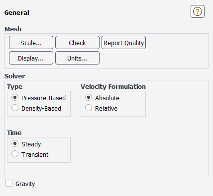
In the Solver group box of the Physics ribbon tab, retain the default selection of the steady pressure-based solver.

Setup → General

19.5.5. Models

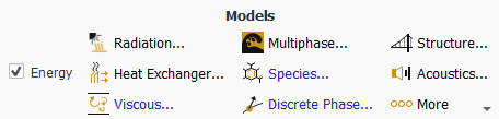
Enable heat transfer by enabling the energy equation.
Physics → Models → Energy
Retain the default k-ω SST turbulence model.
Physics → Models → Viscous...
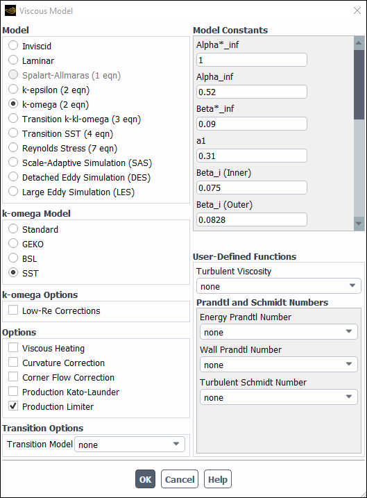
1. Retain the default settings for the k-omega model.
2. Click OK to close the Viscous Model dialog box.
Enable chemical species transport and reaction.
Physics → Models → Species...
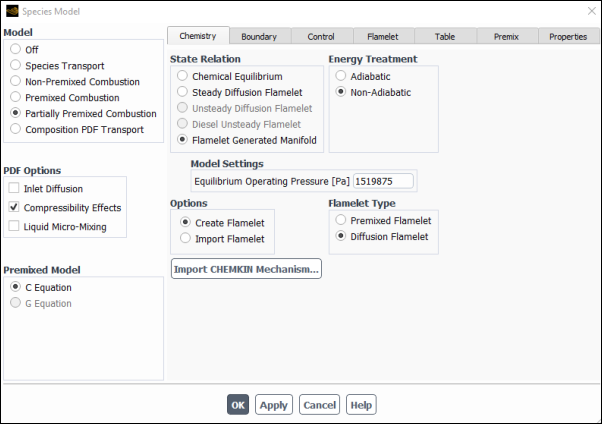
1. Select Partially Premixed Combustion in the Model list.
  The Species Model dialog box will expand to provide further options for the Partially Premixed Combustion model.
2. In the Chemistry Tab,
  1. Select the Flamelet Generated Manifold in the State Relation group box.
  2. Select Non-Adiabatic in the Energy Treatment group box.
  3. Enable Compressibility Effects in the PDF Options group box.
  4. Select Diffusion Flamelet in the Flamelet Type group box.
  5. Set the Equilibrium Operating Pressure (Pa) to 1519875 under Model Settings.
  6. Click Import CHEMKIN Mechanism... to open the Import CHEMKIN Format Mechanism dialog box.
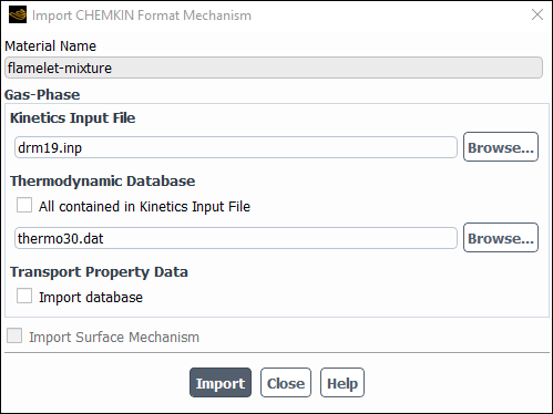
    Select drm19.inp for the Kinetics Input File.
    Select thermo30.dat for the Thermodynamic Database.
    Click Import and close the Import CHEMKIN Format Mechanism dialog box.
3. In the Boundary tab
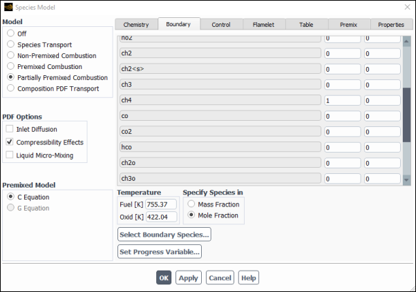
  1. Set ch4 to 1.0.
  2. Set the Fuel to be 755.37 K and the Oxid to be 422.04 K under Temperature
  3. Select Mole Fraction under Specify Species In.
4. In the Control tab, retain the existing settings.
5. In the Flamelet tab,
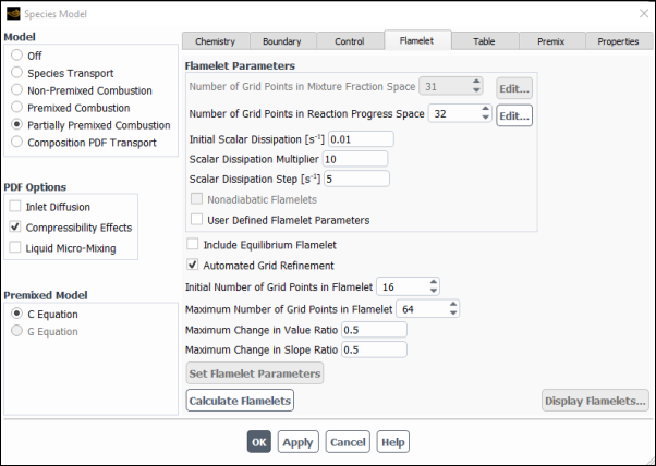
  1. Enable Automated Grid Refinement.
  2. Set the Initial Number of Grid Points in Flamelet to 16.
  3. Click the Calculate Flamelets button.
  4. Then answer Yes and save the flamelet solution into a file named combustor_effusion.fla.gz.
6. In the Table tab
  1. Click the Calculate PDF Table button.
7. Click OK to close the Species Model dialog box.
8. Save the PDF output file (combustor_effusion.pdf.gz).
  File → Write → PDF...
  1. Enter combustor_effusion.pdf.gz for PDF File name.
  2. Click OK to write the file.
Enable Discrete Phase Model
Physics → Models → Discrete Phase...
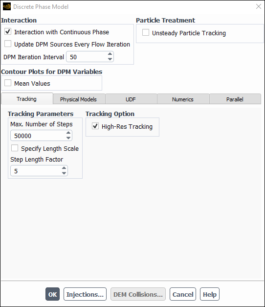
1. Enable the Interaction with Continuous Phase in the Interaction group box.
2. Set the DPM Iteration Interval to 50.
3. In the Numerics Tab
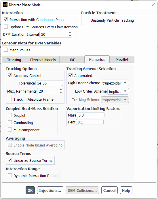
  1. Enable Linearize Source Terms in the Source Terms group box.
  2. Click the Injections button.
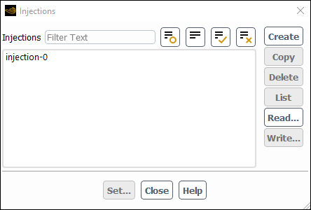
    Click the Create button.
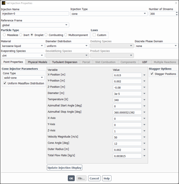
    Select Cone as the injection type and set the Number of Streams to 300.
    Select Droplet as the Particle Type.
    Select kerosene-liquid as the Material and choose ch4 as the Evaporating Species.
    Enable the Uniform Massflow Distribution option.
    Set the X-Position [m] to 0.015 m, Y-Position [m] to 0.002 m, and the Z-Position [m] to -0.08 m.
    Set the Diameter [m] to 3.0E-5m.
    Set the Temperature [K] to 340K.
    Set the Velocity Magnitude [m/s] to 50 m//s.
    Set the Cone Angle to 12 degrees.
    Set the Outer Radius [m] to 0.002m.
    Set the Total Flow Rate [Kg/s] to 0.003815 Kg/s
4. In the Turbulent Dispersion tab
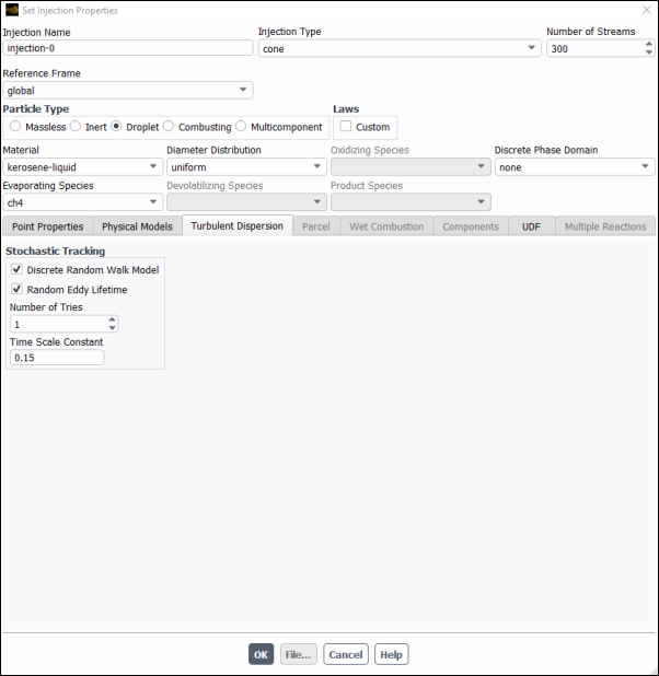
  1. Enable Discrete Random Walk Model and Random Eddy Lifetime.
5. Click OK to close the Set Injection Properties panel.
6. Click Close to close the Injections panel.
7. Click OK to close the Discrete Phase Model panel.

19.5.6. Materials

In this step, you will examine the default settings for the droplet material. This tutorial uses droplet properties copied from theFluent Database. In general, you can modify these or create your own droplet properties for your specific problem as necessary .

Confirm the properties for the mixture materials.
Setup → Materials → Droplet Particle → kerosene-liquid Edit...
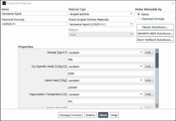
1. Retain the droplet particle properties. In this case, the default properties settings are used so no changes are needed.
2. Close the Create/Edit Materials dialog box.

19.5.7. Operating Conditions

Set the operating pressure.
Setup → Boundary Conditions → Operating Conditions...

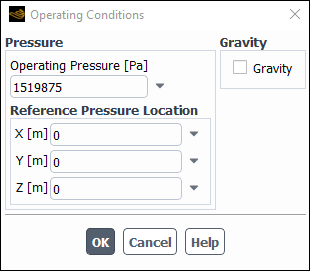
The Operating Conditions dialog box can also be accessed from the Cell Zone Conditions task page.
1. Enter 1519875 Pa for Operating Pressure.
2. Click OK to close the Operating Conditions dialog box.

19.5.8. Boundary Conditions

Set the boundary conditions for the air inlet.
Setup → Boundary Conditions → Inlet → inlet Edit...
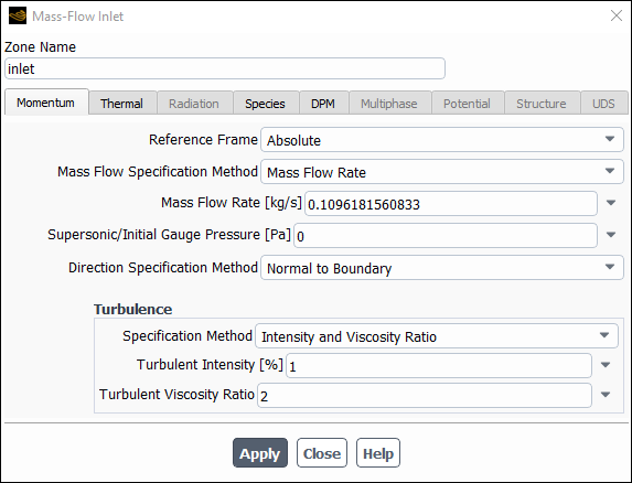
1. Enter inlet for Zone Name.
2. Enter 0.1096181560833 kg/s for Mass Flow Rate.
3. Select Normal to the Boundary from the Direction Specification Method drop-down list.
4. Select Intensity and Viscosity Ratio from the Specification Method drop-down list in the Turbulence group box.
5. Enter 1 for Turbulent Intensity.
6. Enter 2 for Viscosity Ratio.
7. Click the Thermal tab and retain the default value of 755.37222 for Temperature.
8. Click the DPM tab and select escape for the Discrete Phase BC Type.
9. Click Apply and close the Inlet dialog box.

19.5.8.1. Perforated Walls

Setup the perforated walls to model the liner effusion, by reading an input file. .
Setup → Boundary Conditions → Perforated Walls...
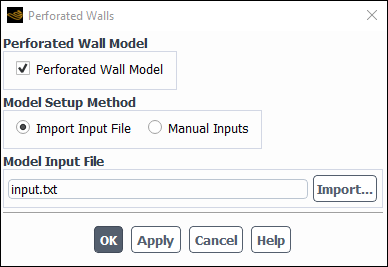
1. Click Import Input File dialog box.
2. Select the file named input.txt.
3. Click Manual Inputs to check the model settings.
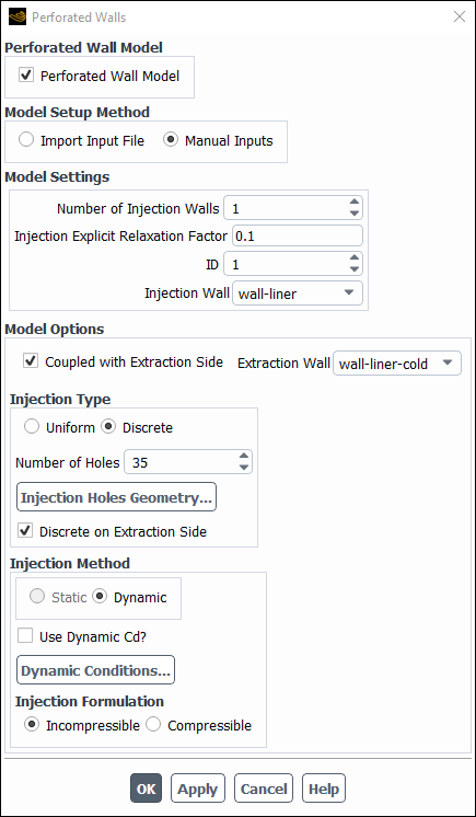
  1. The Number of injection Walls is set to 1.
  2. The Injection Explicit Relaxation Factor is set to 0.1.
  3. Click Injection Holes Geometry... button to view the detailed setup for Injection Holes.
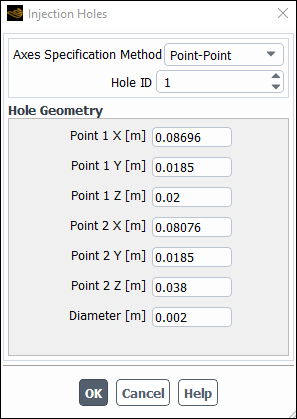
    Click OK to close the Injection Holes dialog box.
  4. Click Dynamic Conditions... button to view the detailed setup for dynamic injection conditions for all the holes.
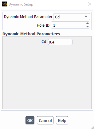
    Click OK to close the Dynamic Setup dialog box.
4. Click OK to close the Perforated Walls dialog box.

19.5.9. Cold Flow Solution

First solve the cold flow through the combustor.

Solution → Solution → Methods...

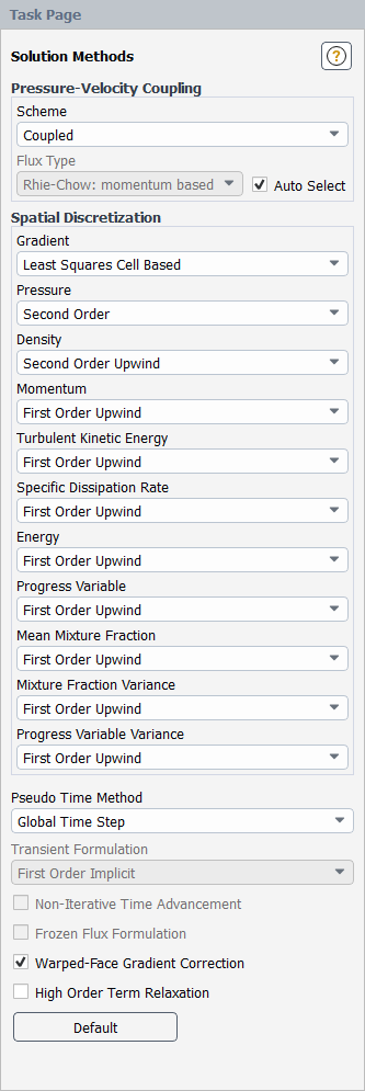
Select Second Order for Pressure, Second Order Upwind for Density and First Order Upwind for the other equations in the Spatial Discretization group box.
Set the solution control parameters. This model combustor is relatively sensitive to the numerical settings, thus to be conservative, low pseudo time explicit relaxation factors are used. Set all the pseudo time explicit relaxation factors to be 0.1, except Body Forces (since there is no body force considered in this case) and Discrete Phase Sources (using the default value of 0.5 since a smaller value may not be able to recover the actual source item). With 0.1 as the relaxation factors, the case may need a greater number of iterations to converge.
Solution → Solution → Controls...

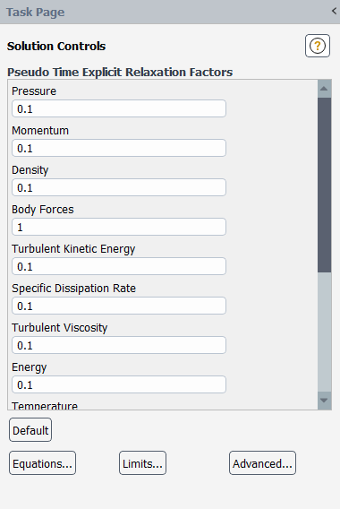
Enter 0.1 for all the Pseudo Time Explicit Relaxation Factors, except for Body Forces and Discrete Phase Sources.
Set the reference pressure method in the TUI.
1. Press Enter in the console to get the command prompt (>).
2. Enter the text commands as shown in the box:
```
define operating-conditions reference-pressure-method 1
  
```
Ensure the plotting of residuals during the calculation.
Solution → Reports → Residuals...
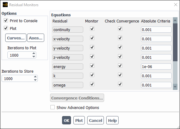
1. Ensure that Plot is enabled in the Options group box.
2. Click OK to close the Residual Monitors dialog box.
Initialize the field variables.
Solution → Initialization
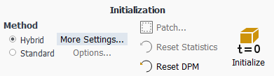
1. Retain the default Hybrid initialization method and click Initialize to initialize the variables.
Save the case file (combustor_effusion.cas.h5).
File → Write → Case...
1. Enter combustor_effusion.cas.h5 for Case File.
2. Ensure that Write Binary Files is enabled to produce a smaller, unformatted binary file.
3. Click OK to close the Select File dialog box.
Run the calculation.
Solution → Run Calculation → Run Calculation...
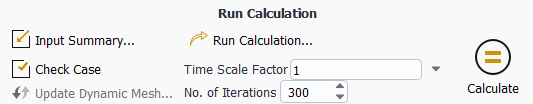
1. Enter 300 for Number of Iterations.
2. Click Calculate.
Save the case and data files (combustor_effusion.cas.h5 and combustor_effusion.dat.h5).
File → Write → Case & Data...
Note: If you choose a file name that already exists in the current folder, Ansys Fluent will ask you to confirm that the previous file is to be overwritten.

19.5.10. Combustion Solution

Now model cooling flow with combustion.

Initialize the Progress Variable variable used for the ignition model.
Solution → Initialization
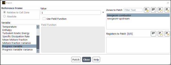
1. Click Patch... to initialize the variables.
2. Select Progress Variable from the Variable list.
3. Enter 1 for the Value.
4. Select newgeom-combustor from the Zones to Patch list.
5. Click Patch and close the Patch dialog box..
Run the calculation.
1. Enter 400 for Number of Iterations.
2. Click Calculate.
Save the case and data files (combustor_effusion.cas.h5 and combustor_effusion.dat.h5).
File → Write → Case & Data...
Note: If you choose a file name that already exists in the current folder, Ansys Fluent will ask you to confirm that the previous file is to be overwritten.

19.5.11. Postprocessing

Review the solution by examining graphical displays of the results.

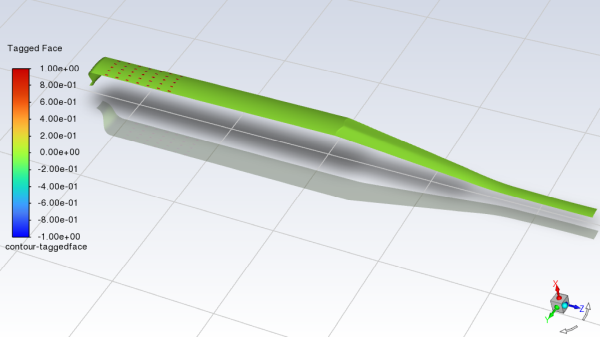
Display effusion hole locations.
Results → Graphics → Contours → New...
1. Enter contour-taggedface for Contour Name.
2. Ensure that Filled is enabled in the Options group box.
3. Select Smooth in the Coloring group box.
4. Select Perforated... and Tagged Face in the Contours of drop-down lists.
5. Select wall-liner and wall-heatsheild from the Surfaces lists.
6. Click Save/Display and close the Contours dialog box.
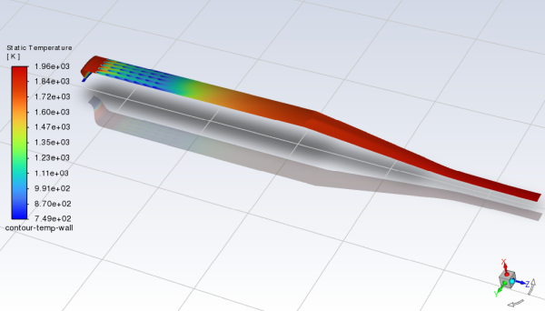
Display filled contours of wall temperature.
Results → Graphics → Contours → New...
1. Enter contour-temp-wall for Contour Name.
2. Ensure that Filled is enabled in the Options group box.
3. Disable Global Range in the Options group box.
4. Select Smooth in the Coloring group box.
5. Select Temperature... and Static Temperature in the Contours of drop-down lists.
6. Select wall-liner and wall-heatsheild from the Surfaces lists.
7. Click Save/Display and close the Contours dialog box.
Create an iso-surface through the combustor geometry.
Results → Surface → Create → Iso-Surface...
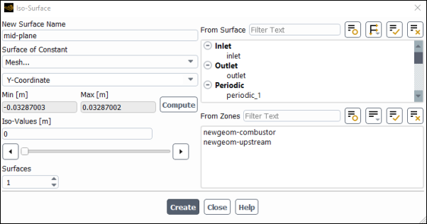
1. Enter mid-plane for Name.
2. Select Mesh... and Y-Coordinate from the Surface of Constant drop-down lists.
3. Click Compute.
  The Min and Max fields display the Y extents of the domain.
4. Enter 0 for the Iso-Values.
5. Click Create and close the Iso-Surface dialog box.
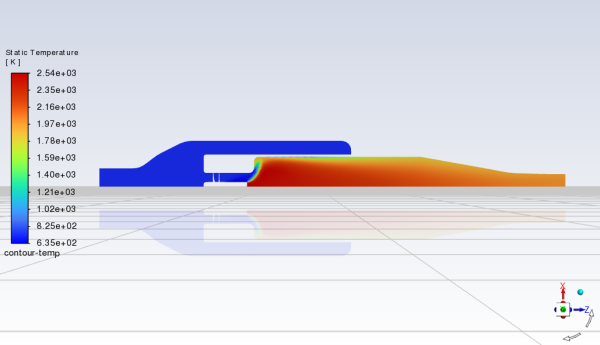
Display filled contours of temperature on a plane.
Results → Graphics → Contours → New...
1. Enter contour-temp for Contour Name.
2. Ensure that Filled is enabled in the Options group box.
3. Select Smooth in the Coloring group box.
4. Select Temperature... and Static Temperature in the Contours of drop-down lists.
5. Select mid-plane from the Surfaces lists.
6. Click Save/Display and close the Contours dialog box.
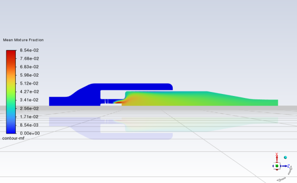
Display filled contours of mean mixture fraction.
Results → Graphics → Contours → New...
1. Enter contour-mf for Contour Name.
2. Ensure that Filled is enabled in the Options group box.
3. Select Smooth in the Coloring group box.
4. Select Pdf... and Mean Mixture Fraction in the Contours of drop-down lists.
5. Select mid-plane from the Surfaces lists.
6. Click Save/Display and close the Contours dialog box.
Save the case file (combustor_effusion.cas.h5).
File → Write → Case...

19.6. Summary

In this tutorial you used Ansys Fluent to model the effusion cooling effects with perforated wall model in a 3D model combustor. Discrete injection type is used here for the effusion cooling injections. The procedures used here for simulation of effusion cooling can be applied to other combustors.